Walmart_Sales_Exploratory_Data_Analysis_Project

🛒 Walmart Sales EDA(Exploratory Data Analysis) Project

General Topics:

Import the libraries
Load the Dataset
Drop Duplicate Rows
Change column format(if need)

import numpy as np
import pandas as pd
import matplotlib.pyplot as plt
import seaborn as sns

df = pd.read_csv(r"D:\B_Data_Anlysist_Project\Python_Projects\02_Walmart_EDA\eda_walmart_sales_dataset.csv")
df.head()

df.info()

<class 'pandas.core.frame.DataFrame'>
RangeIndex: 1000 entries, 0 to 999
Data columns (total 10 columns):
 #   Column         Non-Null Count  Dtype  
---  ------         --------------  -----  
 0   Order ID       1000 non-null   object 
 1   Order Date     1000 non-null   object 
 2   Customer ID    1000 non-null   object 
 3   Customer Name  1000 non-null   object 
 4   City           1000 non-null   object 
 5   Region         1000 non-null   object 
 6   Category       1000 non-null   object 
 7   Quantity       1000 non-null   int64  
 8   Sales          1000 non-null   float64
 9   Profit         1000 non-null   float64
dtypes: float64(2), int64(1), object(7)
memory usage: 78.3+ KB

df.drop_duplicates(inplace= True)

df["Order Date"] = pd.to_datetime(df["Order Date"])

df.info()

<class 'pandas.core.frame.DataFrame'>
RangeIndex: 1000 entries, 0 to 999
Data columns (total 10 columns):
 #   Column         Non-Null Count  Dtype         
---  ------         --------------  -----         
 0   Order ID       1000 non-null   object        
 1   Order Date     1000 non-null   datetime64[ns]
 2   Customer ID    1000 non-null   object        
 3   Customer Name  1000 non-null   object        
 4   City           1000 non-null   object        
 5   Region         1000 non-null   object        
 6   Category       1000 non-null   object        
 7   Quantity       1000 non-null   int64         
 8   Sales          1000 non-null   float64       
 9   Profit         1000 non-null   float64       
dtypes: datetime64[ns](1), float64(2), int64(1), object(6)
memory usage: 78.3+ KB

Q1. Customer Segmentation Challenge:

customer_profit = df.groupby("Customer ID")["Profit"].sum().reset_index()
customer_profit

customer_profit = customer_profit.sort_values(by= "Profit", ascending= False)
customer_profit

top_10_percent_num = int(0.10 * customer_profit.shape[0])
top_10_percent_num

top_10_percent_df = customer_profit.head(top_10_percent_num)
top_10_percent_df

top_df = df[df["Customer ID"].isin(top_10_percent_df["Customer ID"])]
top_df

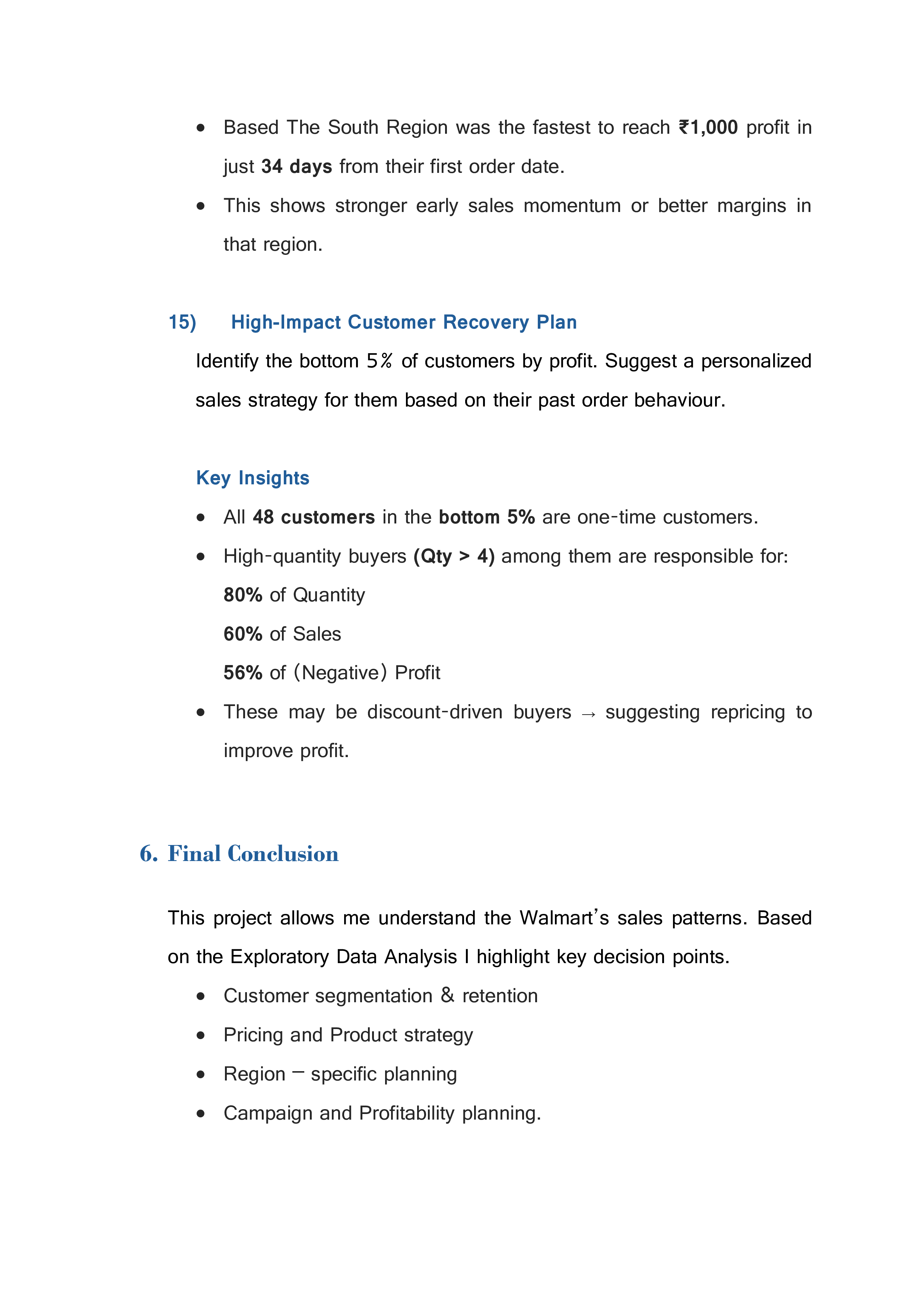
Region column:

region = top_df["Region"].value_counts()
region_index = region.index
region_values = region.values

region = top_df["Region"].value_counts()
region

Region
West     30
East     26
North    25
South    25
Name: count, dtype: int64

sns.barplot(x= region_index, y= region_values)
plt.show

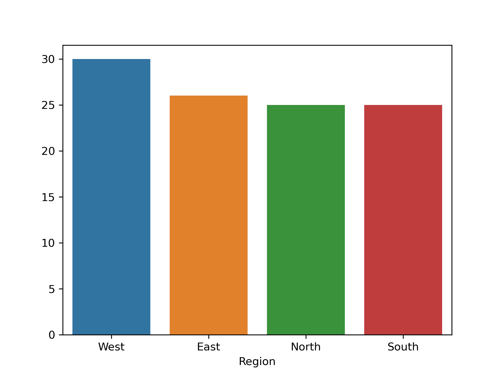
Category column:

category = top_df["Category"].value_counts()
category_index = category.index
category_value = category.values

print(top_df["Category"].value_counts())

Category
Furniture          39
Office Supplies    37
Technology         30
Name: count, dtype: int64

sns.barplot(x= category_index,y= category_value)
plt.show()

print(top_df["City"].value_counts().head(10))

City
South Megan          2
South Alyssamouth    1
Reyesmouth           1
North Sandyfurt      1
South Ashleyhaven    1
Craigport            1
New Stephanie        1
Ricefurt             1
Melissatown          1
New Rachaelhaven     1
Name: count, dtype: int64

Conclusion:

Region: Distribution is fairly even, but [East] has a slight edge.
Category: [Furniture] appears more frequently.
City: One or two cities like [South Megan] show up more than once, but no strong city dominance.

Q2. Monthly Sales Recovery Strategy:

Determine which month in the past year had the lowest overall profit. What specific product category and region contributed most to this loss?

df_loss = pd.DataFrame(df)
df_loss.head()

df_loss["Order Date"].nunique()

df_loss["Year"] = df_loss["Order Date"].dt.year

df_loss["Month"] = df_loss["Order Date"].dt.month

df_loss["Year"].unique()

array([2024, 2023, 2025])

df_loss["Year"].value_counts()

Year
2024    492
2025    275
2023    233
Name: count, dtype: int64

df_2024 = df_loss[df_loss["Year"] == 2024]
df_2024

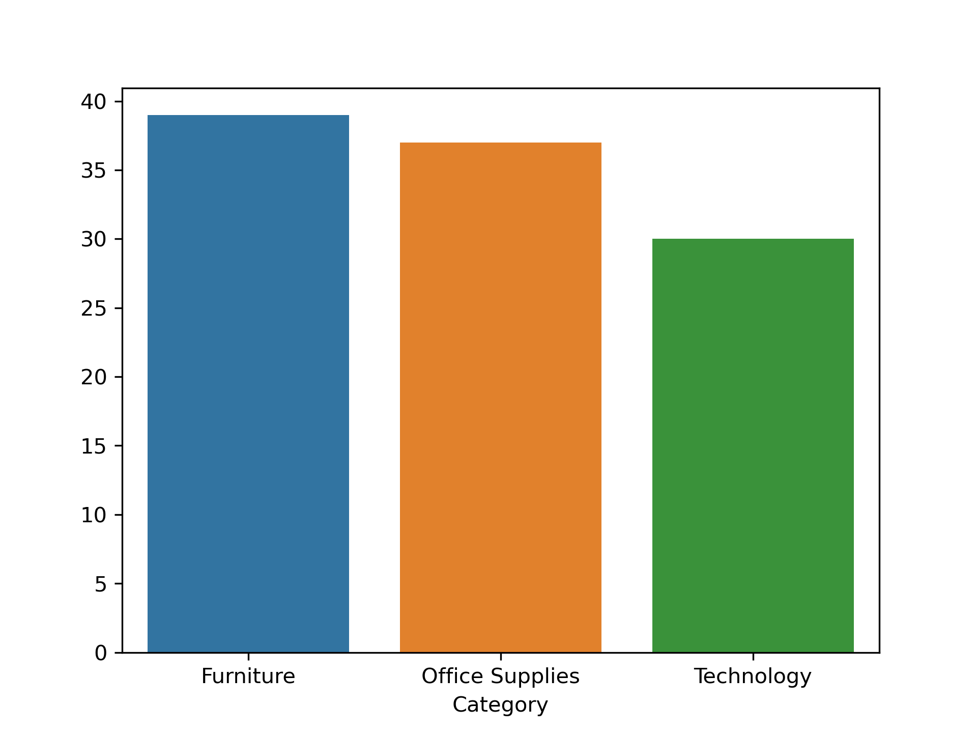
Monthly profit:

df_2024_months = df_2024.groupby("Month")["Profit"].sum().reset_index()
df_2024_months

df_2024_months = df_2024_months.sort_values(by= "Profit", ascending= False)
df_2024_months

sns.barplot(x= df_2024_months["Month"], y= df_2024_months["Profit"])
plt.show()

df_march = df_2024[df_2024["Month"] == 3]
df_march.head()

df_march["Profit"].info()

<class 'pandas.core.series.Series'>
Index: 41 entries, 8 to 993
Series name: Profit
Non-Null Count  Dtype  
--------------  -----  
41 non-null     float64
dtypes: float64(1)
memory usage: 656.0 bytes

df_march["Profit"].sum()

Region wise Distribution:

df_march["Region"].value_counts()

Region
North    13
South    11
West     10
East      7
Name: count, dtype: int64

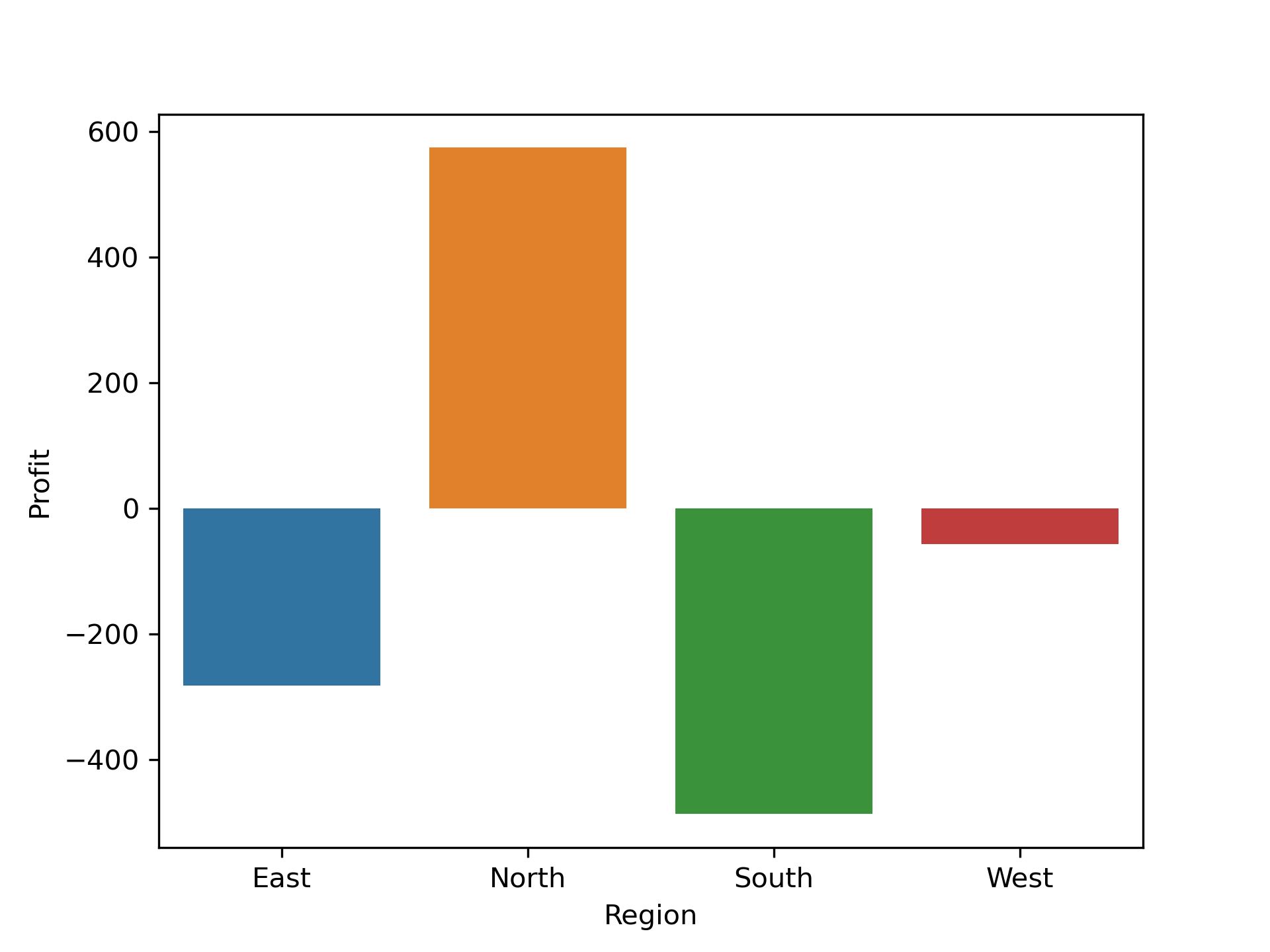
region = df_march.groupby("Region")["Profit"].sum()
region

Region
East    -282.76
North    574.55
South   -486.86
West     -57.15
Name: Profit, dtype: float64

region.index
region.values
sns.barplot(x= region.index, y= region.values)
plt.ylabel("Profit")
plt.show()

Category wise Distribution:

df_march["Category"].value_counts()

Category
Office Supplies    18
Furniture          12
Technology         11
Name: count, dtype: int64

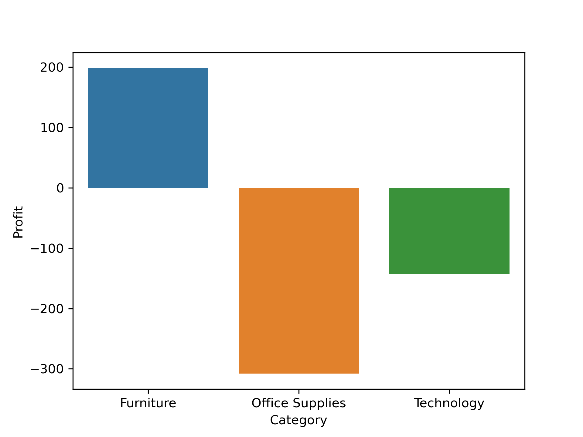
Category = df_march.groupby("Category")["Profit"].sum()
Category

Category
Furniture          199.04
Office Supplies   -307.96
Technology        -143.30
Name: Profit, dtype: float64

Category.index
Category.values
sns.barplot(x= Category.index, y= Category.values)
plt.ylabel("Profit")
plt.show()

Both wise Distribution:

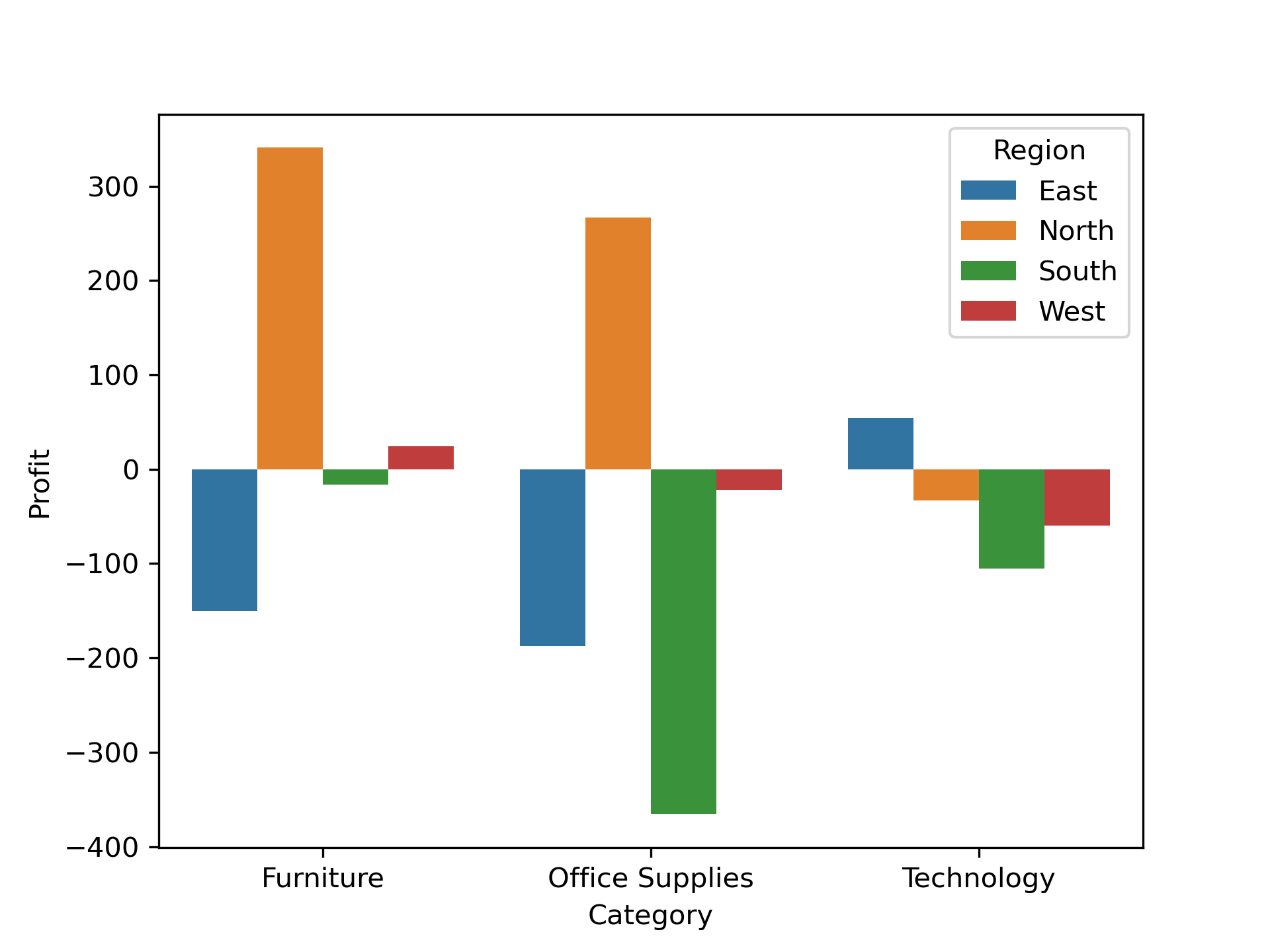
df_march.groupby(["Category","Region"])["Profit"].sum()

Category         Region
Furniture        East     -150.12
                 North     340.85
                 South     -16.23
                 West       24.54
Office Supplies  East     -187.05
                 North     266.55
                 South    -365.34
                 West      -22.12
Technology       East       54.41
                 North     -32.85
                 South    -105.29
                 West      -59.57
Name: Profit, dtype: float64

grouped = df_march.groupby(["Category", "Region"])["Profit"].sum().reset_index()

sns.barplot(x="Category", y="Profit", hue="Region", data=grouped)
plt.show()

Conclusion:

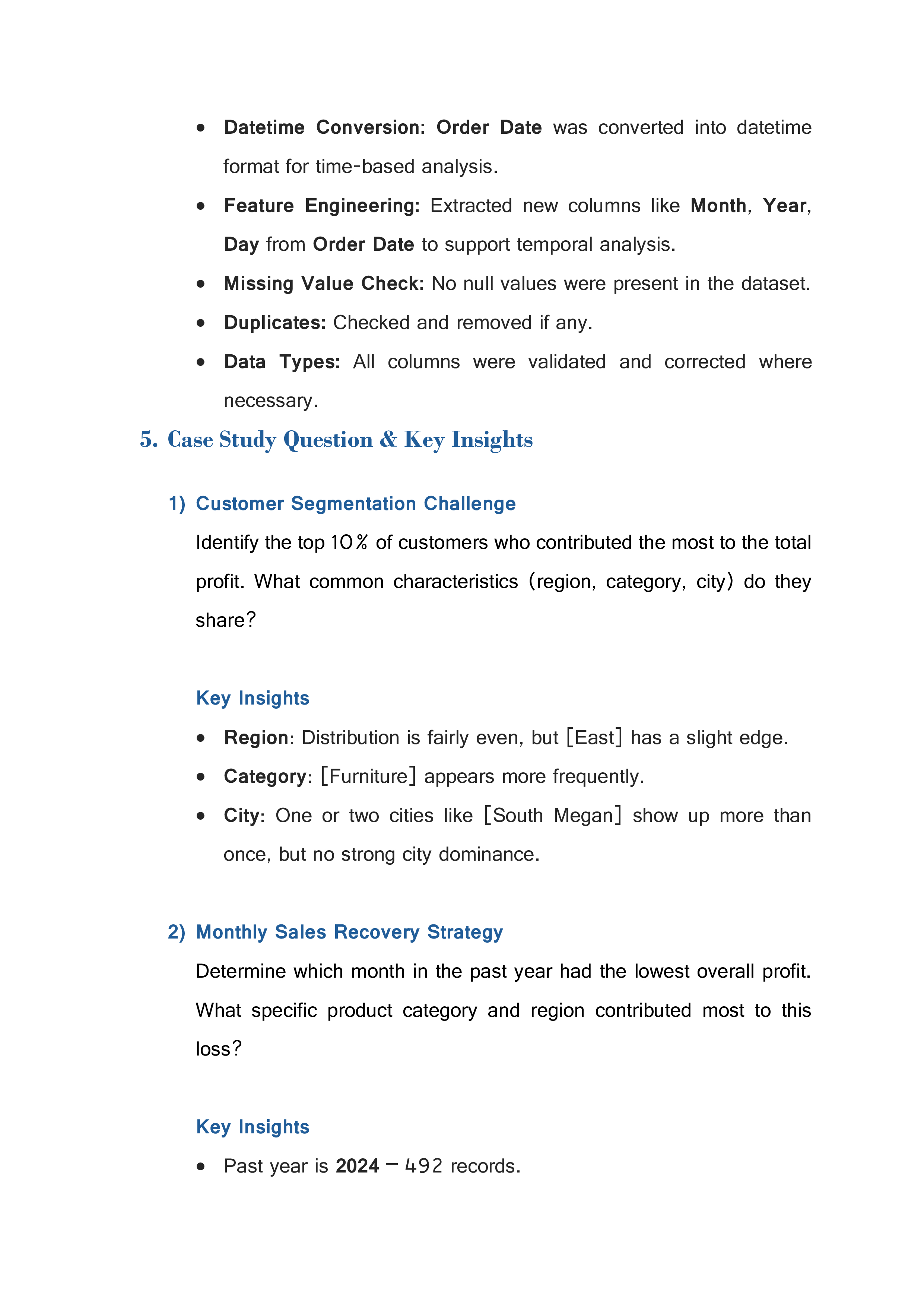
Past year is 2024 – 492 records.
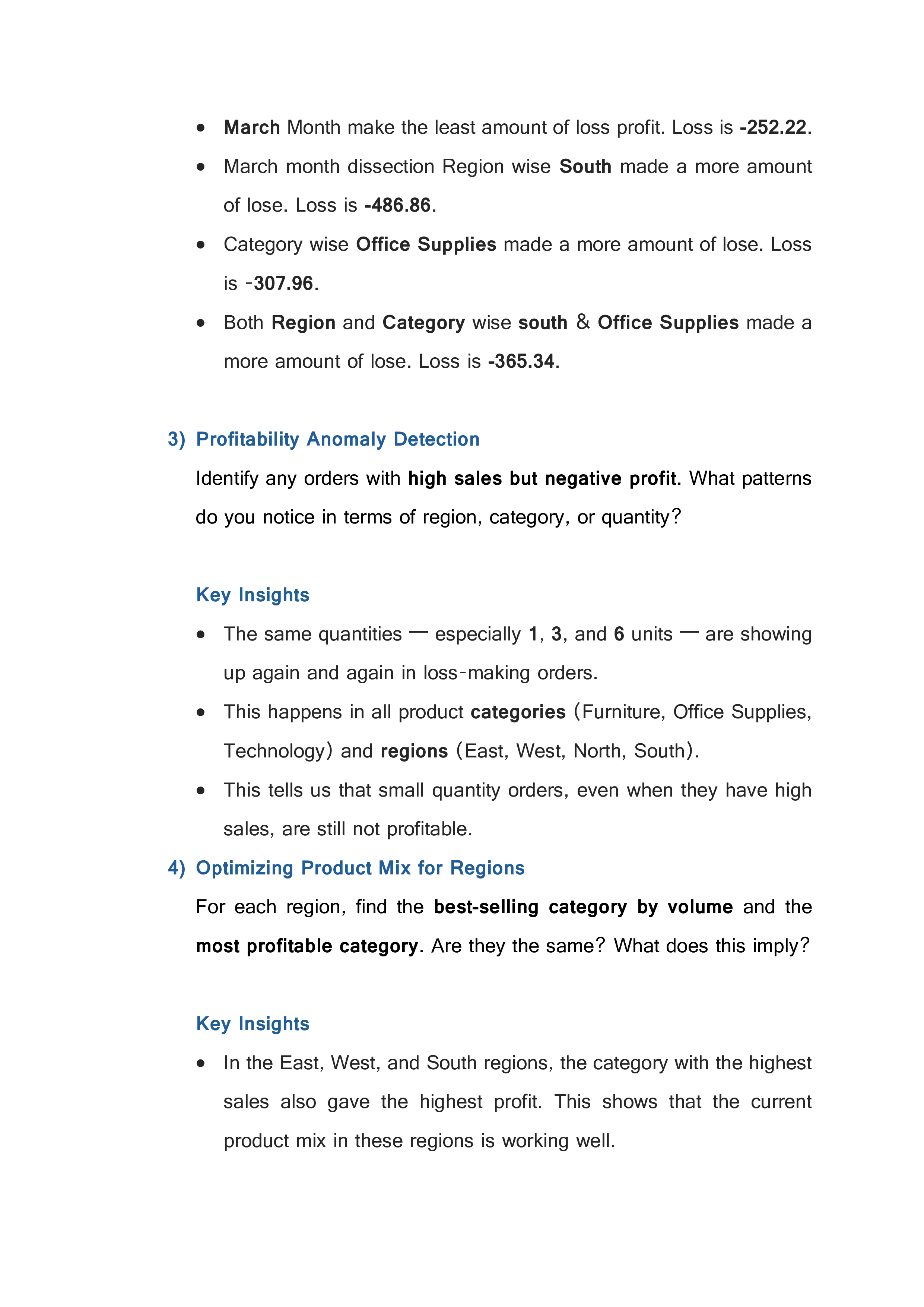
March Month make the least amount of loss profit. Loss is -252.22.
March month dissection Region wise South made a more amount of lose. Loss is -486.86.
Category wise Office Supplies made a more amount of lose. Loss is -307.96.
Both Region and Category wise south & Office Supplies made a more amount of lose. Loss is -365.34.

Q3. Profitability Anomaly Detection:

Identify any orders with high sales but negative profit. What patterns do you notice in terms of region, category, or quantity?

df_anomaly = pd.DataFrame(df)
df_anomaly

df_neg_profit = df_anomaly[df_anomaly["Profit"] < 0]
df_neg_profit

df_neg_profit.groupby("Category").agg({"Category" : "count"})

df_neg_profit["Quantity"].unique()

array([7, 8, 6, 2, 1, 9, 3, 5, 4], dtype=int64)

Furniture Distribution:

df_count_furniture = df_neg_profit[df_neg_profit["Category"] == "Furniture"].groupby("Quantity")["Profit"].count()
df_count_furniture

Quantity
  16
  10
  14
   7
   9
  19
  14
  15
  11
Name: Profit, dtype: int64

df_neg_profit_furniture = df_neg_profit[df_neg_profit["Category"] == "Furniture"].groupby("Quantity")["Profit"].sum()
df_neg_profit_furniture

Quantity
  -802.44
  -577.02
  -805.80
  -389.89
  -630.29
 -1181.15
  -607.38
  -688.04
  -532.80
Name: Profit, dtype: float64

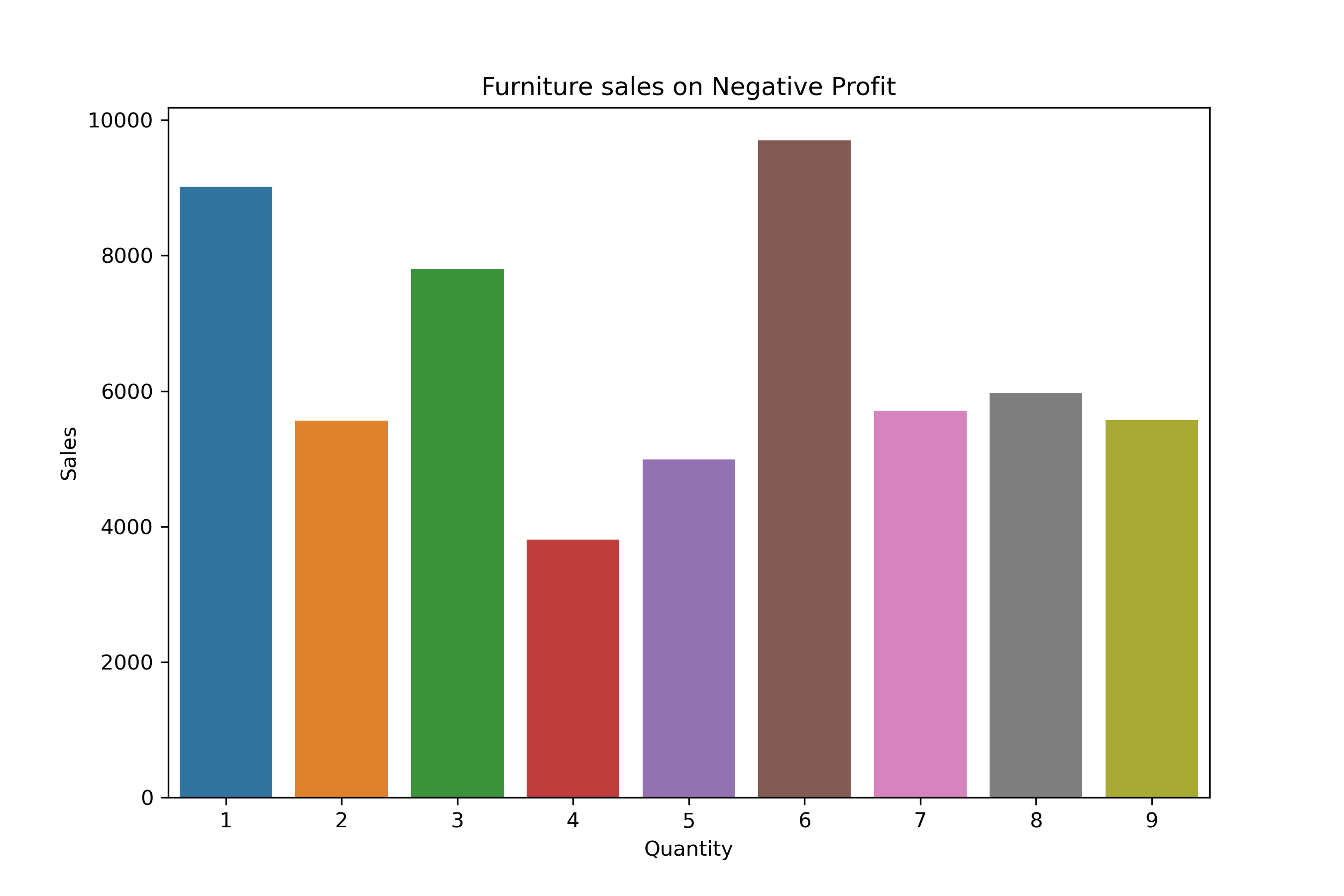
df_furniture = df_neg_profit[df_neg_profit["Category"] == "Furniture"].groupby("Quantity")["Sales"].sum()
df_furniture

Quantity
  9013.62
  5562.43
  7801.78
  3806.66
  4987.83
  9700.03
  5712.62
  5971.68
  5570.56
Name: Sales, dtype: float64

plt.figure(figsize = (9,6))
sns.barplot(x= df_furniture.index, y= df_furniture.values)
plt.title("Furniture sales on Negative Profit")
plt.ylabel("Sales")
plt.show()

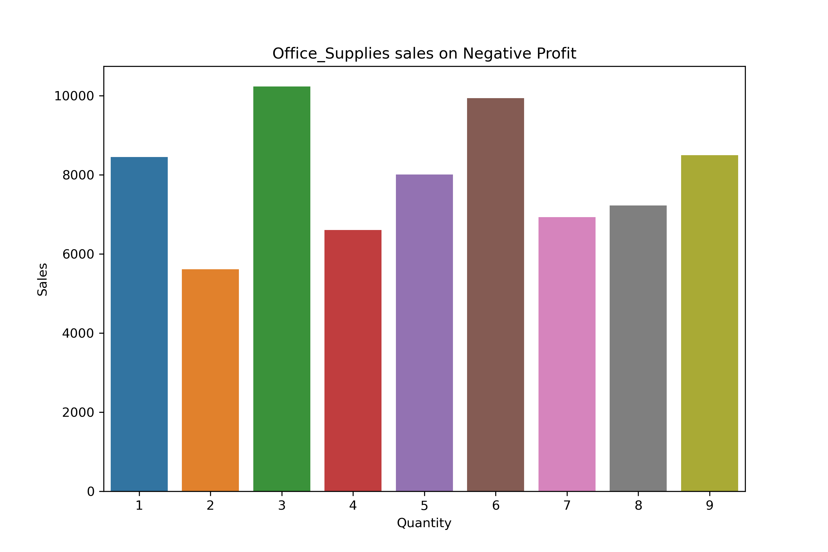
Office_Suppliers Distribution:

df_count_Office_Supplies = df_neg_profit[df_neg_profit["Category"] == "Office Supplies"].groupby("Quantity")["Profit"].count()
df_count_Office_Supplies

Quantity
  16
  13
  21
  12
  17
  18
  14
  15
  16
Name: Profit, dtype: int64

df_neg_Office_Supplies = df_neg_profit[df_neg_profit["Category"] == "Office Supplies"].groupby("Quantity")["Profit"].sum()
df_neg_Office_Supplies

Quantity
  -876.00
  -661.01
  -924.51
  -628.67
  -691.39
 -1191.58
  -562.95
  -725.70
  -582.02
Name: Profit, dtype: float64

df_Office_Supplies = df_neg_profit[df_neg_profit["Category"] == "Office Supplies"].groupby("Quantity")["Sales"].sum()
df_Office_Supplies

Quantity
   8454.98
   5615.46
  10234.87
   6603.31
   8006.98
   9938.60
   6935.57
   7224.52
   8494.63
Name: Sales, dtype: float64

plt.figure(figsize = (9,6))
sns.barplot(x= df_Office_Supplies.index, y= df_Office_Supplies.values)
plt.title("Office_Supplies sales on Negative Profit")
plt.ylabel("Sales")
plt.show()

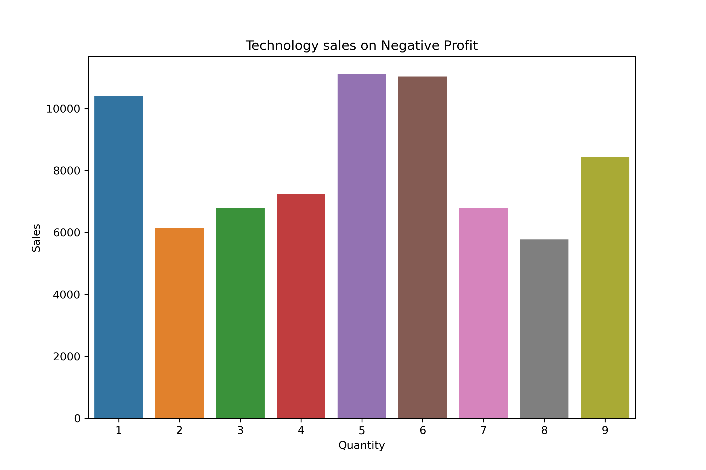
Technology Distribution:

df_count_Technology = df_neg_profit[df_neg_profit["Category"] == "Technology"].groupby("Quantity")["Profit"].count()
df_count_Technology

Quantity
  19
  14
  14
  16
  19
  20
  14
  11
  14
Name: Profit, dtype: int64

df_neg_Technology = df_neg_profit[df_neg_profit["Category"] == "Technology"].groupby("Quantity")["Profit"].sum()
df_neg_Technology

Quantity
  -965.17
  -710.43
  -812.00
  -604.46
 -1283.44
  -960.39
  -625.54
  -518.92
  -884.20
Name: Profit, dtype: float64

df_Technology = df_neg_profit[df_neg_profit["Category"] == "Technology"].groupby("Quantity")["Sales"].sum()
df_Technology

Quantity
  10400.94
   6155.91
   6783.78
   7235.92
  11130.52
  11033.73
   6800.03
   5772.87
   8434.57
Name: Sales, dtype: float64

plt.figure(figsize = (9,6))
sns.barplot(x= df_Technology.index, y= df_Technology.values)
plt.title("Technology sales on Negative Profit")
plt.ylabel("Sales")
plt.show()

East Region Distribution:

df_neg_profit["Region"].unique()

array(['South', 'East', 'North', 'West'], dtype=object)

df_count_East = df_neg_profit[df_neg_profit["Region"] == "East"].groupby("Quantity")["Profit"].count()
df_count_East

Quantity
  14
  10
  10
   7
  11
  19
  14
  13
  14
Name: Profit, dtype: int64

df_profit_East = df_neg_profit[df_neg_profit["Region"] == "East"].groupby("Quantity")["Profit"].sum()
df_profit_East

Quantity
  -929.15
  -454.48
  -545.82
  -517.64
  -451.72
 -1240.21
  -704.56
  -669.10
  -681.08
Name: Profit, dtype: float64

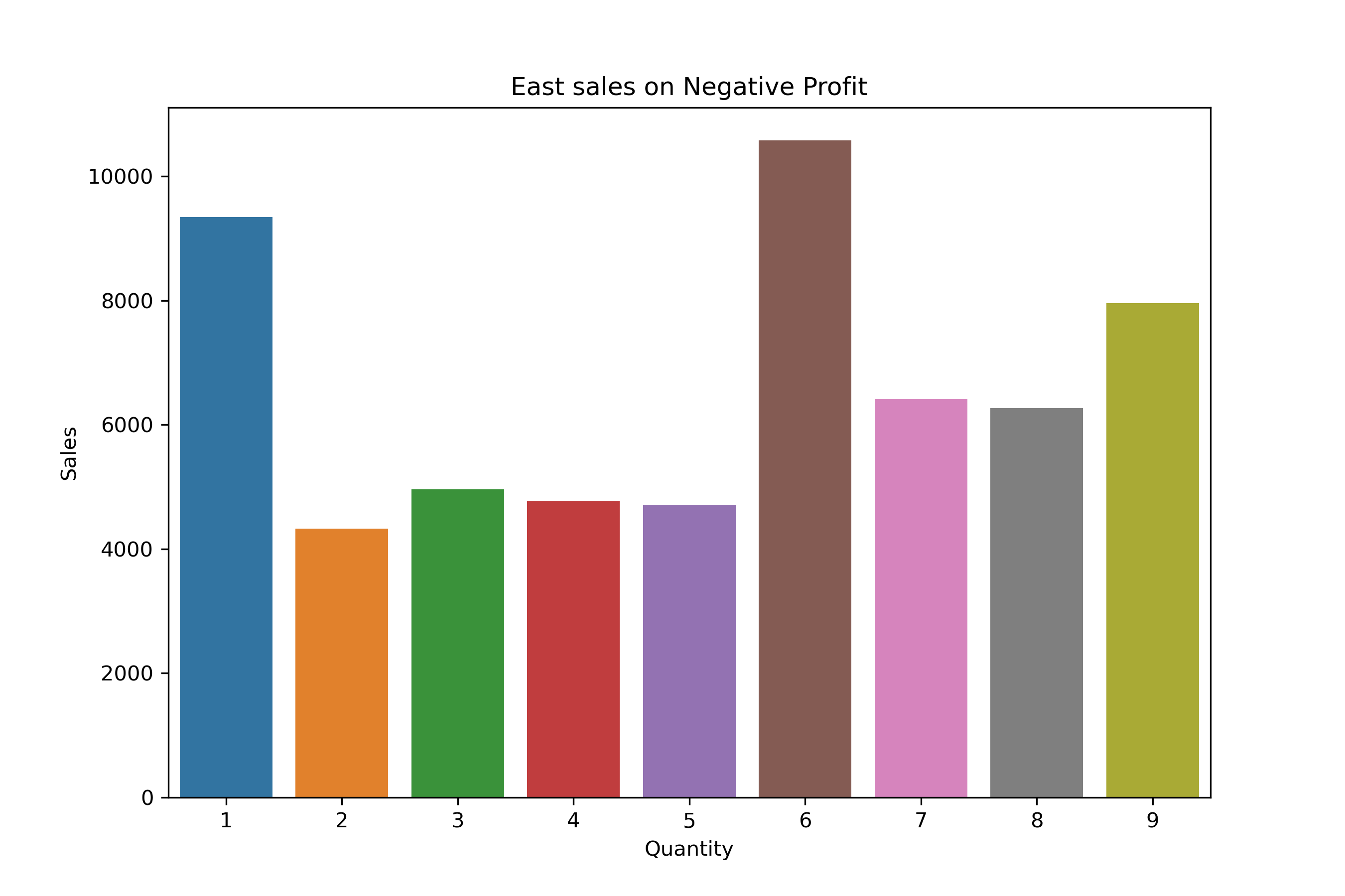
df_sales_East = df_neg_profit[df_neg_profit["Region"] == "East"].groupby("Quantity")["Sales"].sum()
df_sales_East

Quantity
   9344.71
   4328.10
   4958.74
   4776.51
   4709.89
  10578.75
   6412.53
   6265.65
   7954.16
Name: Sales, dtype: float64

plt.figure(figsize = (9,6))
sns.barplot(x= df_sales_East.index, y= df_sales_East.values)
plt.title("East sales on Negative Profit")
plt.ylabel("Sales")
plt.show()

West Region Distribution:

df_profit_West = df_neg_profit[df_neg_profit["Region"] == "West"].groupby("Quantity")["Profit"].count()
df_profit_West

Quantity
  12
   9
  15
  14
  13
  13
  10
  15
  10
Name: Profit, dtype: int64

df_profit_West = df_neg_profit[df_neg_profit["Region"] == "West"].groupby("Quantity")["Profit"].sum()
df_profit_West

Quantity
 -329.90
 -150.25
 -735.72
 -701.62
 -590.07
 -688.36
 -389.78
 -794.10
 -305.97
Name: Profit, dtype: float64

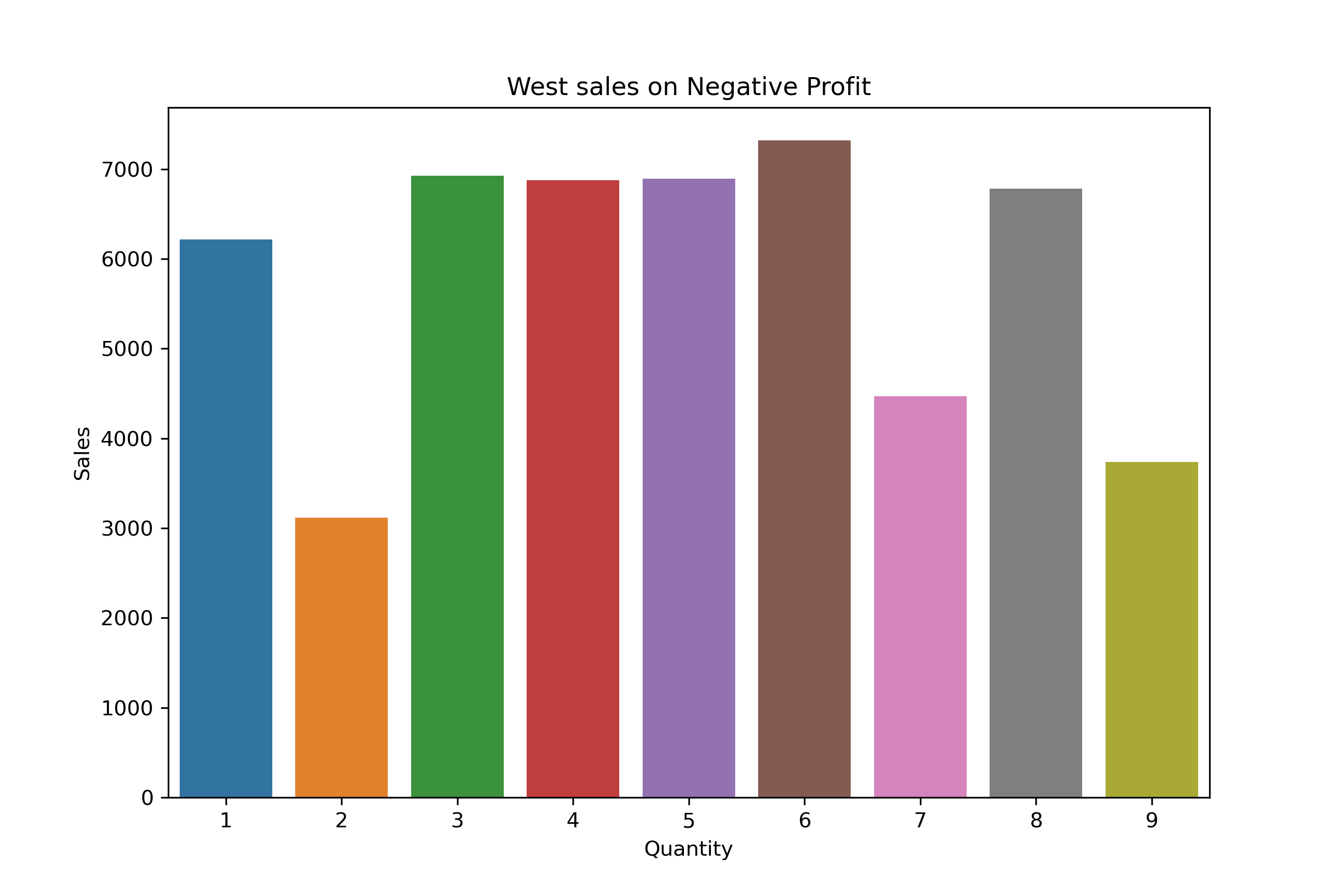
df_sales_West = df_neg_profit[df_neg_profit["Region"] == "West"].groupby("Quantity")["Sales"].sum()
df_sales_West

Quantity
  6215.65
  3118.75
  6925.78
  6878.59
  6895.15
  7319.91
  4470.00
  6783.22
  3736.70
Name: Sales, dtype: float64

plt.figure(figsize = (9,6))
sns.barplot(x= df_sales_West.index, y= df_sales_West.values)
plt.title("West sales on Negative Profit")
plt.ylabel("Sales")
plt.show()

North Region Distribution:

df_profit_North = df_neg_profit[df_neg_profit["Region"] == "North"].groupby("Quantity")["Profit"].count()
df_profit_North

Quantity
  13
   6
  14
   5
   7
   9
   6
   9
  11
Name: Profit, dtype: int64

df_profit_North = df_neg_profit[df_neg_profit["Region"] == "North"].groupby("Quantity")["Profit"].sum()
df_profit_North

Quantity
 -764.34
 -285.40
 -730.11
 -133.06
 -623.66
 -402.46
 -162.61
 -299.10
 -827.33
Name: Profit, dtype: float64

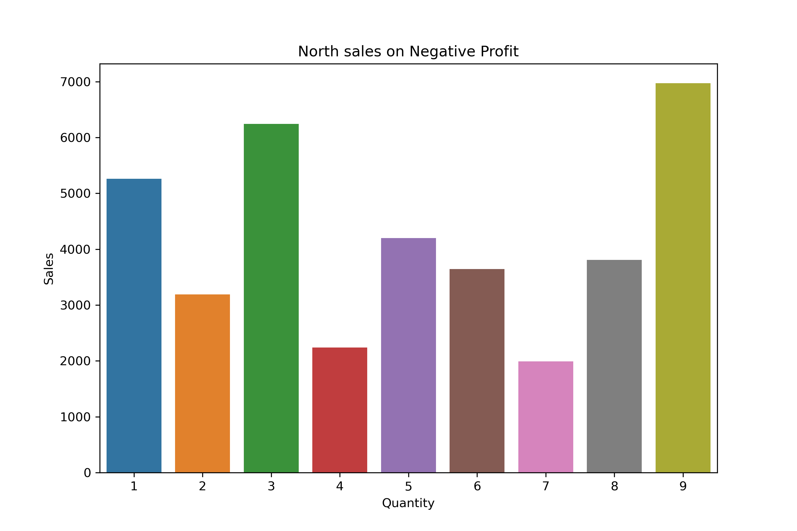
df_profit_North = df_neg_profit[df_neg_profit["Region"] == "North"].groupby("Quantity")["Sales"].sum()
df_profit_North

Quantity
  5257.83
  3190.53
  6243.89
  2241.93
  4197.23
  3641.99
  1992.01
  3807.97
  6971.56
Name: Sales, dtype: float64

plt.figure(figsize = (9,6))
sns.barplot(x= df_profit_North.index, y= df_profit_North.values)
plt.title("North sales on Negative Profit")
plt.ylabel("Sales")
plt.show()

South Region Distribution:

df_profit_South = df_neg_profit[df_neg_profit["Region"] == "South"].groupby("Quantity")["Profit"].count()
df_profit_South

Quantity
  12
  12
  10
   9
  14
  16
  12
   4
   6
Name: Profit, dtype: int64

df_profit_South = df_neg_profit[df_neg_profit["Region"] == "South"].groupby("Quantity")["Profit"].sum()
df_profit_South

Quantity
  -620.22
 -1058.33
  -530.66
  -270.70
  -939.67
 -1002.09
  -538.92
  -170.36
  -184.64
Name: Profit, dtype: float64

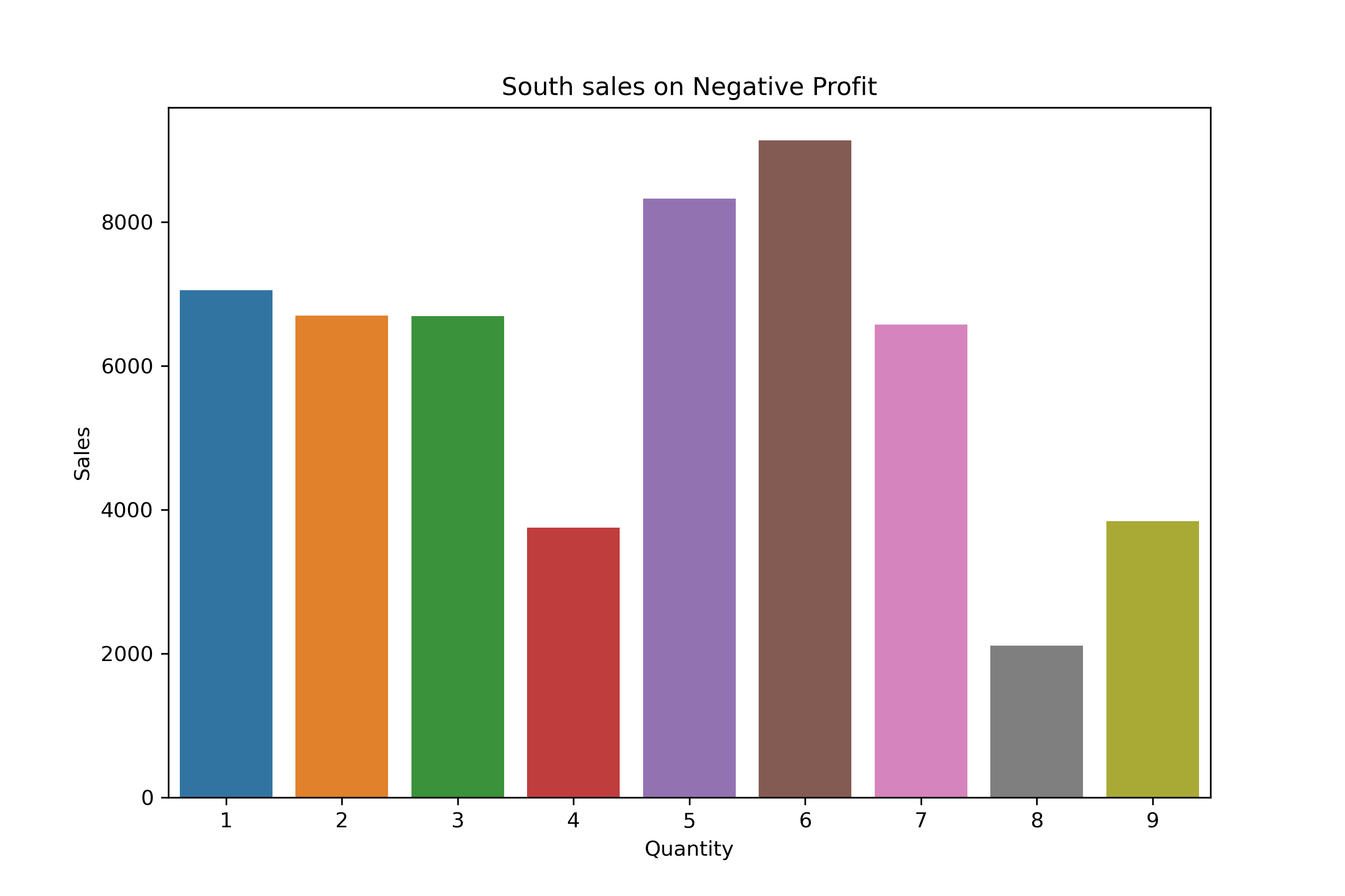
df_profit_South = df_neg_profit[df_neg_profit["Region"] == "South"].groupby("Quantity")["Sales"].sum()
df_profit_South

Quantity
  7051.35
  6696.42
  6692.02
  3748.86
  8323.06
  9131.71
  6573.68
  2112.23
  3837.34
Name: Sales, dtype: float64

plt.figure(figsize = (9,6))
sns.barplot(x= df_profit_South.index, y= df_profit_South.values)
plt.title("South sales on Negative Profit")
plt.ylabel("Sales")
plt.show()

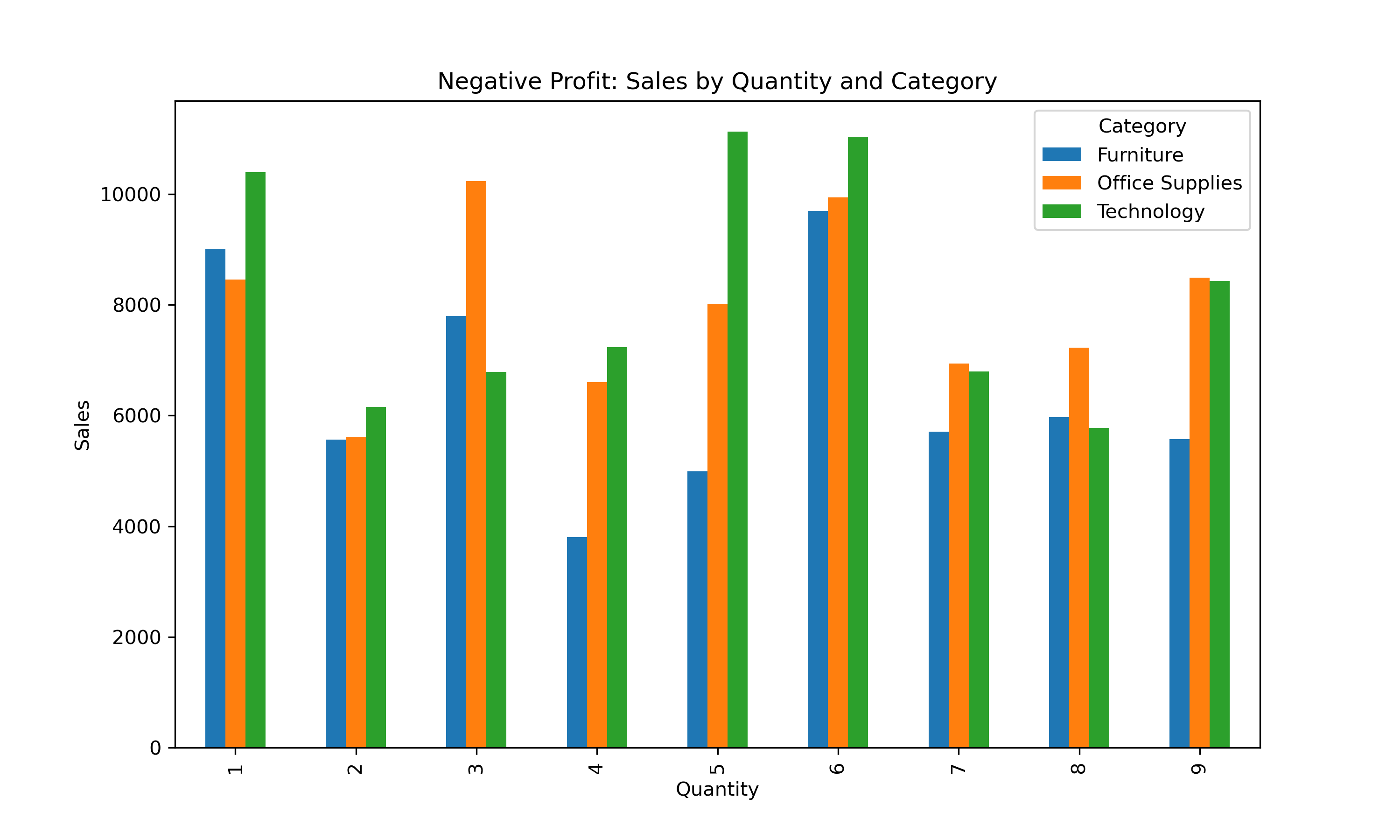
Overall Visualization:

category_sales = df_neg_profit.pivot_table(index="Quantity", columns="Category", values="Sales", aggfunc="sum")
category_sales.plot(kind="bar", figsize=(10,6))
plt.title("Negative Profit: Sales by Quantity and Category")
plt.ylabel("Sales")
plt.show()

region_quantity = df_neg_profit.pivot_table(index="Quantity", columns="Region", values="Sales", aggfunc="sum")
sns.heatmap(region_quantity, annot=True, cmap="YlOrRd", fmt=".0f")
plt.title("Sales with Negative Profit by Quantity and Region")
plt.show()

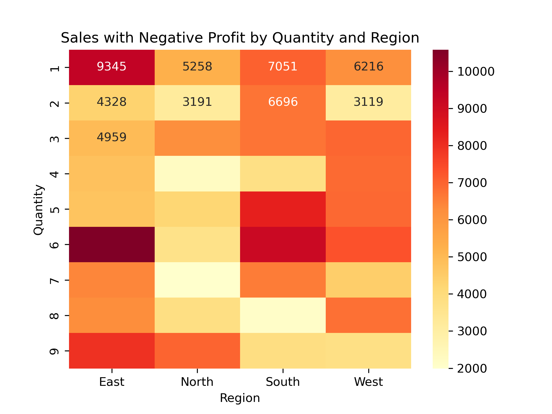
Conclusion:

The same quantities — especially 1, 3, and 6 units — are showing up again and again in loss-making orders.
This happens in all product categories (Furniture, Office Supplies, Technology).
It also happens in all regions (East, West, North, South).
This tells us that small quantity orders, even when they have high sales, are still not profitable.

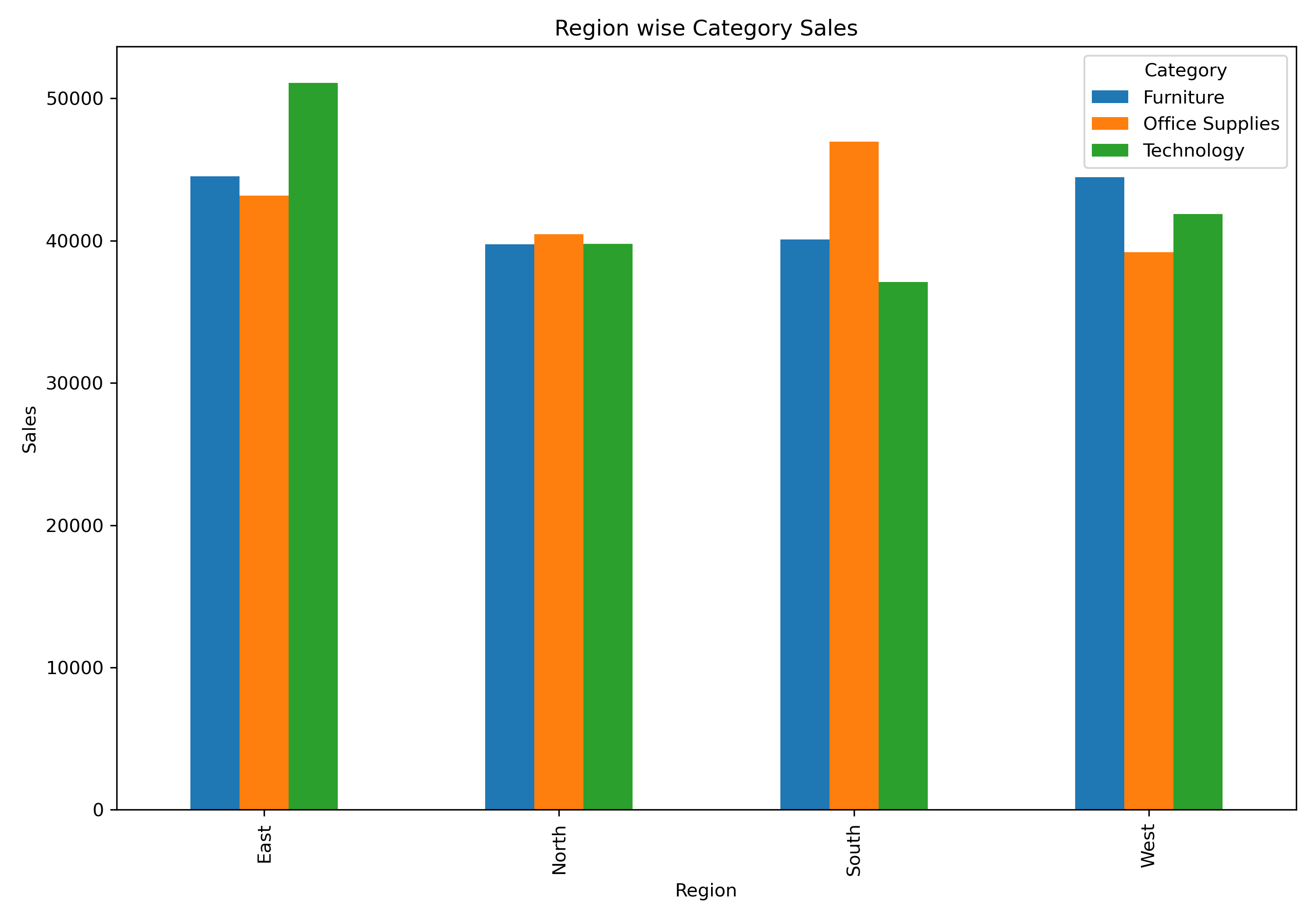
Q4. Optimizing Product Mix for Regions:

For each region, find the best-selling category by volume and the most profitable category. Are they the same? What does this imply?

df_product_mix = pd.DataFrame(df)
df_product_mix.head()

df_product_mix.groupby(["Region","Category"])["Sales"].sum()

Region  Category       
East    Furniture          44515.40
        Office Supplies    43166.97
        Technology         51097.55
North   Furniture          39738.54
        Office Supplies    40463.24
        Technology         39787.34
South   Furniture          40073.94
        Office Supplies    46950.11
        Technology         37103.00
West    Furniture          44470.98
        Office Supplies    39181.65
        Technology         41876.95
Name: Sales, dtype: float64

df_sales = df_product_mix.pivot_table(index= "Region", columns= "Category", values= "Sales", aggfunc= "sum")
df_sales

df_sales.plot(kind= "bar", figsize= (10,7))
plt.title("Region wise Category Sales")
plt.ylabel("Sales")
plt.tight_layout()
plt.show()

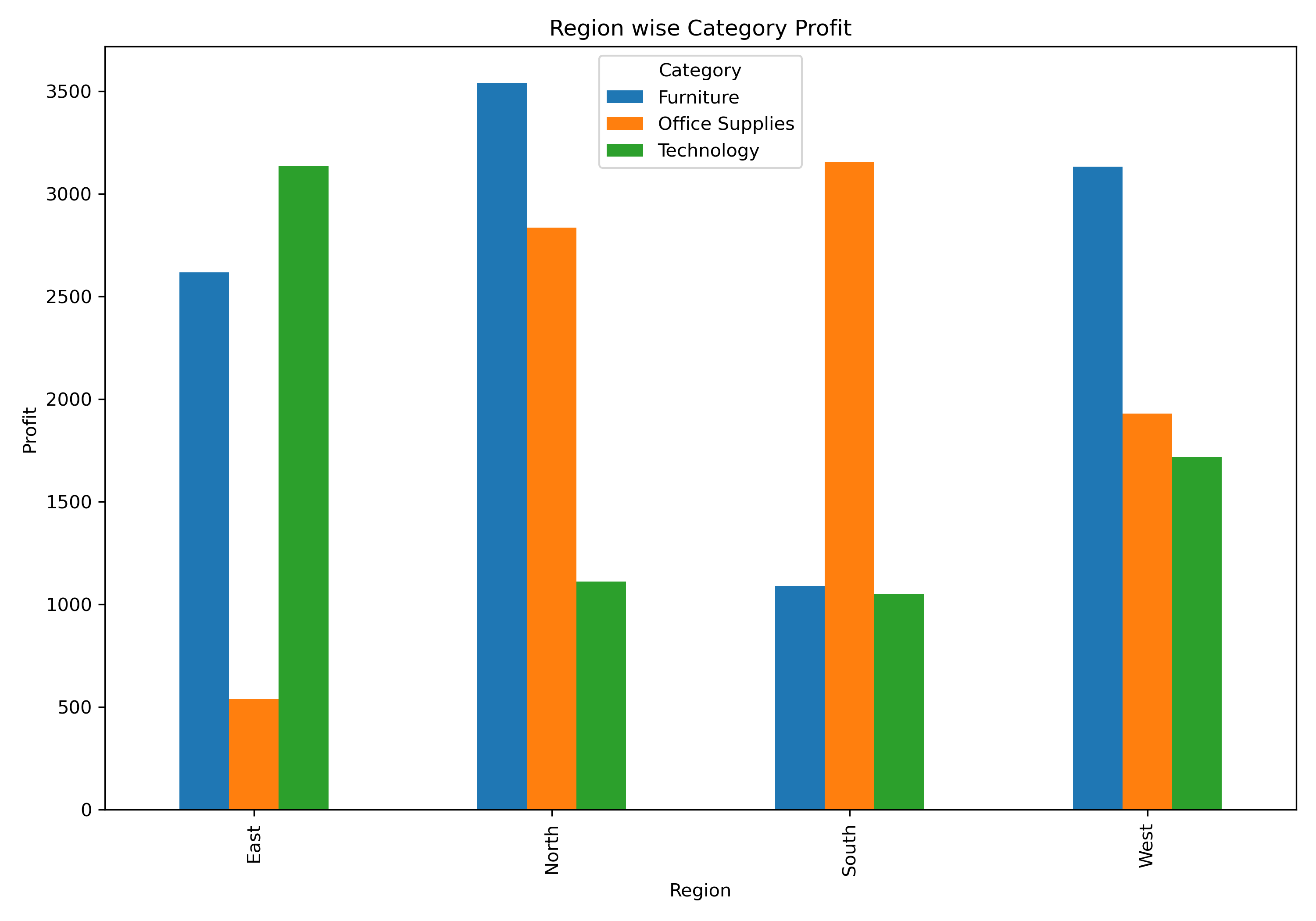
df_profit = df_product_mix.pivot_table(index= "Region", columns= "Category", values= "Profit", aggfunc= "sum")
df_profit

df_profit.plot(kind= "bar", figsize= (10,7))
plt.title("Region wise Category Profit")
plt.ylabel("Profit")
plt.tight_layout()
plt.show()

df_north_office = df_product_mix[(df_product_mix["Region"] == "North") & (df_product_mix["Category"] == "Office Supplies")]
df_north_office

df_north_neg = df_north_office[df_north_office["Profit"] < 0]
df_north_neg

office_positive_profit = df_north_office.groupby("Quantity")["Profit"].sum()
sum(office_positive_profit.values)

office_negative_profit = df_north_neg.groupby("Quantity")["Profit"].sum()
sum(office_negative_profit.values)

df_north_furniture = df_product_mix[(df_product_mix["Region"] == "North") & (df_product_mix["Category"] == "Furniture")]
df_north_furniture

df_north_fur_neg = df_north_office[df_north_office["Profit"] < 0]
df_north_fur_neg

Furniture_positive_profit = df_north_furniture.groupby("Quantity")["Profit"].sum()
sum(Furniture_positive_profit.values)

Furniture_negative_profit = df_north_fur_neg.groupby("Quantity")["Profit"].sum()
sum(Furniture_negative_profit.values)

Conclusion:

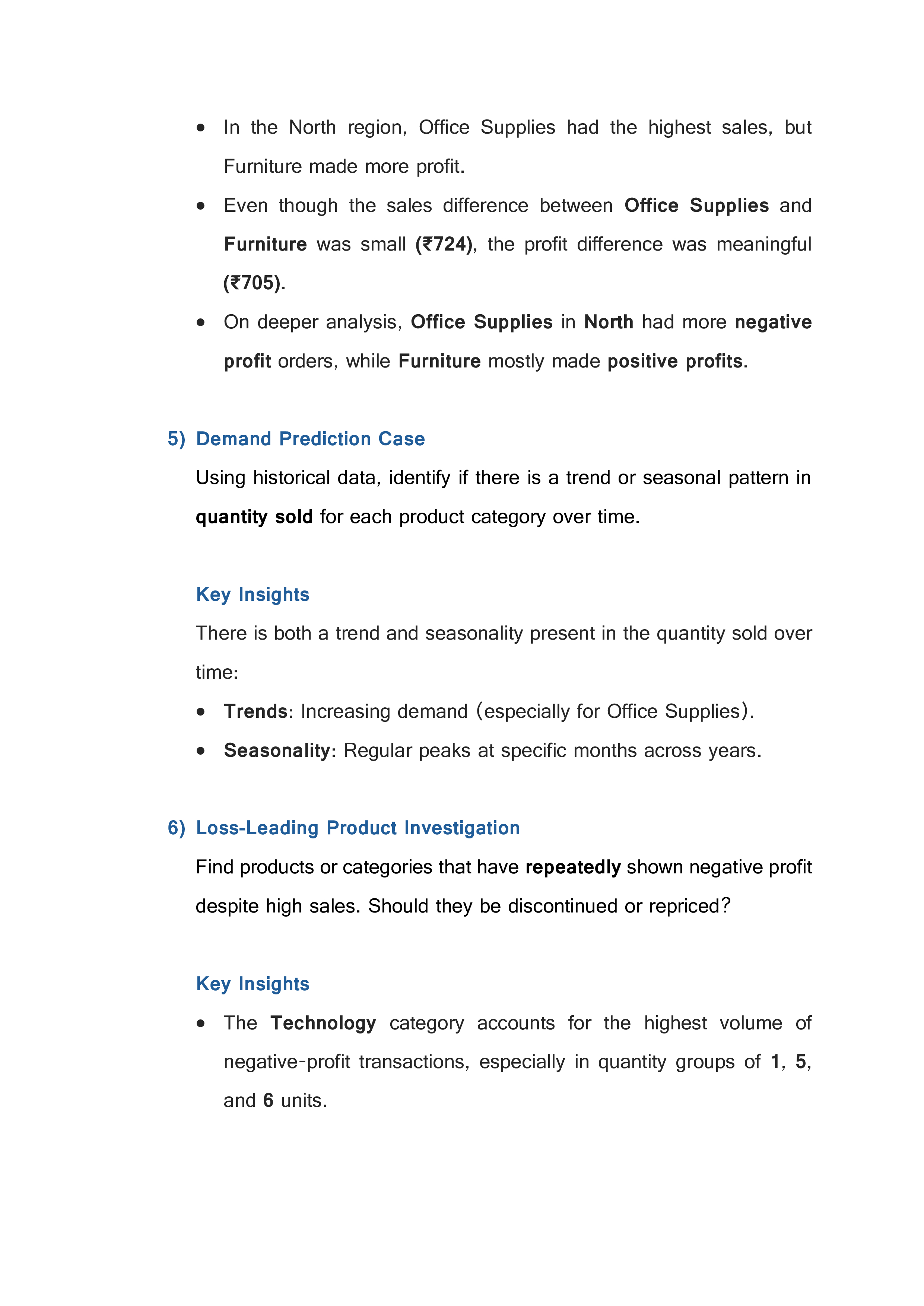
In the East, West, and South regions, the category with the highest sales also gave the highest profit. This shows that the current product mix in these regions is working well.
In the North region, Office Supplies had the highest sales, but Furniture made more profit.
Even though the sales difference between Office Supplies and Furniture was small (₹724), the profit difference was meaningful (₹705).
On deeper analysis, Office Supplies in North had more negative profit orders, while Furniture mostly made positive profits.

Q5. Demand Prediction Case:

Using historical data, identify if there is a trend or seasonal pattern in quantity sold for each product category over time.

df_trend_season = pd.DataFrame(df)
df_trend_season.head()

df_trend_season["Order Date"] = pd.to_datetime(df_trend_season["Order Date"])

df_trend_season["Year"] = df_trend_season["Order Date"].dt.year

df_trend_season["Month"] = df_trend_season["Order Date"].dt.month

df_trend_season["Year-Month"] = df_trend_season["Order Date"].dt.to_period("M")

monthly_trend = df_trend_season.groupby(['Year-Month', 'Category'])['Quantity'].sum().reset_index()
monthly_trend

pivot_df = monthly_trend.pivot(index='Year-Month', columns='Category', values='Quantity')
pivot_df

pivot_df.plot(figsize=(12,6), marker='o')
plt.title("Monthly Quantity Sold by Category")
plt.ylabel("Total Quantity Sold")
plt.xlabel("Month")
plt.xticks(rotation=45)
plt.grid(True)
plt.tight_layout()
plt.show()

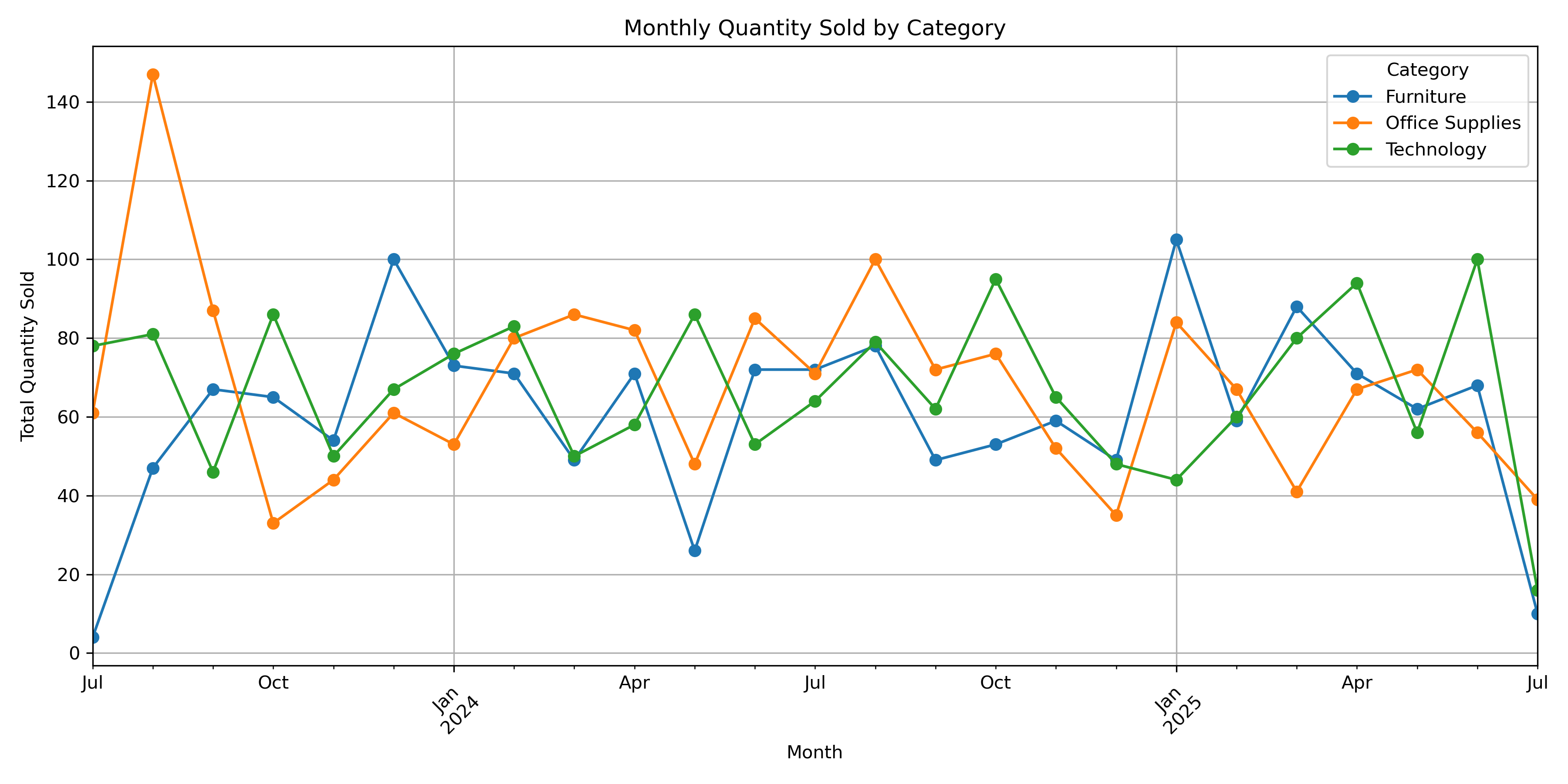
Conclusion:

There is both a trend and seasonality present in the quantity sold over time:

Trends: Increasing demand (especially for Office Supplies).
Seasonality: Regular peaks at specific months across years.

Q6. Loss-Leading Product Investigation:

Find products or categories that have repeatedly shown negative profit despite high sales. Should they be discontinued or repriced?

df_high_sales = pd.DataFrame(df)
df_high_sales.head()

neg_profit = df_high_sales[df_high_sales["Profit"] < 0]
neg_profit

neg_profit.groupby("Category")["Sales"].sum()

Category
Furniture          58127.21
Office Supplies    71508.92
Technology         73748.27
Name: Sales, dtype: float64

neg_profit.groupby("Category")["Profit"].sum()

Category
Furniture         -6214.81
Office Supplies   -6843.83
Technology        -7364.55
Name: Profit, dtype: float64

tech_sort = neg_profit[neg_profit["Category"] == "Technology"]
tech_sort

tech_sort.groupby("Quantity").agg({
    "Quantity" : "count",
    "Sales" : "sum",
    "Profit" : "sum"
}).rename(columns= {"Quantity" : "Order_count"}).reset_index()

tot = tech_sort.groupby(["Quantity"])["Sales"].sum()
tot_sum = sum(tot)
per = (tot.values/tot_sum)*100

Conclusion:

The Technology category accounts for the highest volume of negative-profit transactions, especially in quantity groups of 1,5, and 6 units.
These three quantity buckets alone contribute 45% of loss transactions, indicating that these sales are frequent and significant.
Since these products are selling well (high sales count), it’s more financially sound to reprice them (increase unit price, reduce discount) rather than discontinue them.

Q7. Regional Sales Consistency:

Which region shows the most stable monthly sales performance over time? Use standard deviation or coefficient of variation to support your analysis.

df_std_cv = pd.DataFrame(df)
df_std_cv.head()

df_std_cv["Order Date"] = pd.to_datetime(df_std_cv["Order Date"])

df_std_cv["month_year"] = df_std_cv["Order Date"].dt.to_period("M")

monthly_sales = df_std_cv.groupby(["Region", "month_year"])["Sales"].sum().reset_index()
monthly_sales

region_sales = monthly_sales.groupby("Region")["Sales"].agg(["mean","std"]).reset_index()
region_sales

region_sales["cv"] = region_sales["std"] / region_sales["mean"]

region_sales.sort_values(by= "cv")

Conclusion:

Based on the coefficient of variation (CV) for monthly sales across regions, the North region has the most stable sales performance over time (CV = 0.36).
This indicates less fluctuation in monthly sales, making it the most consistent region in terms of sales.

Q8. Customer Retention Analysis:

Based on Customer ID, find the number of repeats vs. one-time customers. How does their average profit and sales differ?

df_customer = pd.DataFrame(df)

df_customer["Order Date"] = pd.to_datetime(df_customer["Order Date"])

df_customer.head()

customer_count = df_customer["Customer ID"].value_counts()

df_customer["customer_type"] = df_customer["Customer ID"].apply(lambda x : "repeat" if customer_count[x] > 1 else "one_time")

df_customer["customer_type"].value_counts()

customer_type
one_time    912
repeat       88
Name: count, dtype: int64 ```python customer_summary = df_customer.groupby("customer_type")[["Sales","Profit"]].sum() customer_summary ```

customer_summary["per_sales"] = round((customer_summary["Sales"]/ customer_summary["Sales"].sum())*100, 2)

customer_summary["per_profit"] = round((customer_summary["Profit"]/ customer_summary["Profit"].sum())*100, 2)

customer_summary

Conclusion:

Out of all customers, only a small portion are repeat customers, and they contribute ~9% of sales and ~10.5% of profit.
The majority of revenue is currently driven by one-time customers, showing a potential gap in customer retention.
There is no significant profitability difference between repeat and one-time buyers, indicating a possible opportunity to re-engage one-time buyers into becoming repeat customers.

Q9. Bulk Buying Patterns:

Are their specific cities or regions where customers consistently buy in higher quantities than average? What product categories are driving this?

df_cit_reg = pd.DataFrame(df)

region_agg = df_cit_reg.groupby("Region")[["Quantity"]].agg(["count","std","mean"]).reset_index()

region_agg["total_avg"] = df_cit_reg["Quantity"].mean()

a = df_cit_reg["City"].value_counts().reset_index()
a.columns = ["City", "count"]
b = a[a["count"] > 1]

city_filter = df_cit_reg[df_cit_reg["City"].isin(b["City"])]

city_agg = city_filter.groupby("City")[["Quantity"]].agg(["count","mean","std"]).reset_index()

city_agg["total_avg"] = df_cit_reg["Quantity"].mean()

Conclusion:

The East and West regions show slightly above-average bulk buying behavior, with mean quantities above the overall average (4.898).
Standard deviation across regions is relatively consistent, indicating stable purchasing patterns.
City-level analysis was inconclusive, as most cities appeared only once in the dataset and do not provide enough volume to draw meaningful conclusions.

Q10. Sales Efficiency Score:

Create a new metric: Profit per Unit Sold. Rank cities based on this efficiency. What actionable insights can Walmart take?

df_pro_per_unit = pd.DataFrame(df)
df_pro_per_unit.head()

df_city_cal = df_pro_per_unit.groupby("City")[["Quantity", "Profit"]].sum().reset_index()
df_city_cal.columns = ["City", "Quantity", "Profit"]
df_city_cal

df_city_cal["Per_unit"] = df_city_cal["Profit"] / df_city_cal["Quantity"]
df_city_cal

top_10_profit = df_city_cal.sort_values(by= "Per_unit", ascending= False).head(10)
top_10_profit

bottom_10_profit = df_city_cal.sort_values(by= "Per_unit").head(10)
bottom_10_profit

Conclusion:

A new metric, Profit per Unit Sold, was created to evaluate the sales efficiency of each city.

The top 10 cities generate high profit per unit, indicating strong product mix or premium customer segments.
The bottom 10 cities show low or negative efficiency, possibly due to high volume of low-margin items or higher return rates.

Actionable insights for Walmart:
Focus on expanding profitable categories in high-efficiency cities.
In low-efficiency cities, re-evaluate pricing, optimize product assortment, or address operational inefficiencies.

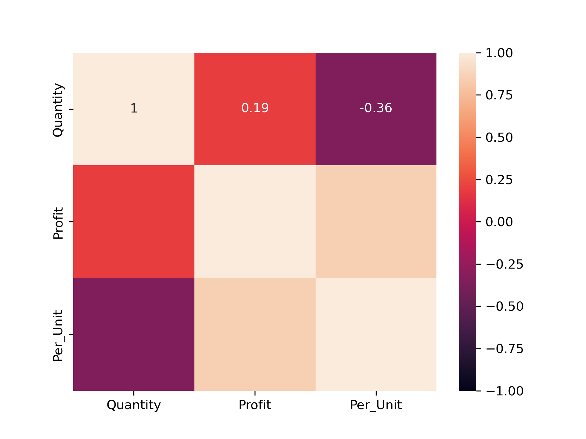
Q11. Sales Efficiency Score:

Is there a negative correlation between quantity sold and profit per unit in any region or category? What does this suggest?

df_neg_reg = pd.DataFrame(df)

region_regg = df_neg_reg.groupby("Region")[["Quantity","Profit"]].sum().reset_index()
region_regg.columns = ["Region", "Quantity", "Profit"]
region_regg["Per_Unit"] = region_regg["Profit"] / region_regg["Quantity"]
region_regg

a = region_regg.drop("Region", axis= 1)

region_cor = a.corr()
sns.heatmap(region_cor,vmin= -1, vmax= 1 ,annot= True)
plt.show()

cat_regg = df_neg_reg.groupby("Category")[["Quantity","Profit"]].sum().reset_index()
cat_regg.columns = ["Category", "Quantity", "Profit"]
cat_regg["Per_Unit"] = cat_regg["Profit"] / cat_regg["Quantity"]
cat_regg

b = cat_regg.drop("Category", axis= 1)

cat_cor = b.corr()
sns.heatmap(cat_cor,vmin= -1, vmax= 1 ,annot= True)
plt.show()

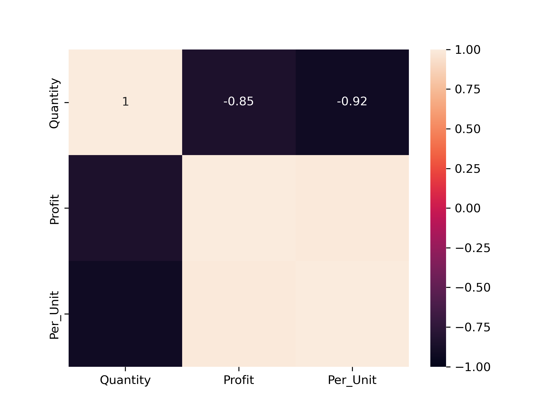
Conclusion:

According to the region segment – Yes negative correlation between quantity sold and profit per unit is occurring and negative correlation value = -0.36.
According to the Category segment – Yes negative correlation between quantity sold and profit per unit is occurring and Occurring negative correlation value = -0.92.

Q12. Campaign Impact Simulation:

Assume Walmart ran a 10% discount campaign in August 2024. Recalculate profit for that month and evaluate how the campaign would have affected overall profitability.

df_aug_10 = pd.DataFrame(df)
df_aug_10.head()

df_extract_aug = df_aug_10[(df_aug_10["Order Date"] >= "2024-08-01") & (df_aug_10["Order Date"] <= "2024-08-31")]
df_extract_aug.reset_index().head()

august_10_per = df_extract_aug["Profit"] - (df_extract_aug["Profit"] / 100) * 10
august_10_per.head()

seperate_aug = df_aug_10["Profit"].sum() - df_extract_aug["Profit"].sum()
seperate_aug

overall_10_profit = seperate_aug + august_10_per.sum()
overall_10_profit

without_dis = round(df_aug_10["Profit"].sum() / df_aug_10["Profit"].count(), 2)
without_dis

with_10_dis = round(overall_10_profit / df_aug_10["Profit"].count(), 2)
with_10_dis

Conclusion:

Before 10% discount: ₹25.86 profit/order

After discount: ₹25.78 profit/order

Impact = only ₹0.08 difference

This indicates that Walmart can safely run such discount campaigns without significantly harming profitability.
If the discount leads to even a small boost in sales volume, the overall profit may actually increase.

Q13. Return Risk Zones:

If high-quantity orders with low profit are considered risky for returns, which region shows the highest risk exposure?

df_return_risk = pd.DataFrame(df)

df_return_risk.groupby(["Region", "Quantity"])[["Quantity", "Profit"]].sum()

sep_east = df_return_risk[(df_return_risk["Region"] == "East") & (df_return_risk["Quantity"] == 9)]
q_east = sep_east["Quantity"].sum()
p_east = sep_east["Profit"].sum()

sep_east = df_return_risk[(df_return_risk["Region"] == "South") & (df_return_risk["Quantity"] == 9)]
q_south = sep_east["Quantity"].sum()
p_south = sep_east["Profit"].sum()

sep_east = df_return_risk[(df_return_risk["Region"] == "North") & (df_return_risk["Quantity"] == 8)]
q_north = sep_east["Quantity"].sum()
p_north = sep_east["Profit"].sum()

sep_east = df_return_risk[(df_return_risk["Region"] == "West") & (df_return_risk["Quantity"] == 8)]
q_west = sep_east["Quantity"].sum()
p_west = sep_east["Profit"].sum()

join = pd.DataFrame({
    "Quantity_count" : [q_east, q_south, q_north, q_west],
    "Profit_sum" : [p_east, p_south, p_north, p_west]
             }, index= ["east", "south", "north", "west"])

join["Profit_perc"] = (join["Profit_sum"] / join["Profit_sum"].sum()) * 100
join

Conclusion:

Based on the Region segmentation East region has Quantity count is 270, total profit is 289.05, and percentage is 11.09% contribution.

East has high quantity but very low profit, so it is most at risk.

Q14. Return Risk Zones:

Calculate how many days (based on order date) it took each region to cross a cumulative profit of ₹5,000. Who was fastest?

df_time = df.copy()
df_time.head()

filter_1 = df_time.groupby(["Region", "Order Date"])["Profit"].sum().reset_index()
filter_1 = filter_1.sort_values(["Region", "Order Date"])
filter_1["cumsum"] = filter_1.groupby("Region")["Profit"].cumsum()

filter_2 = filter_1[filter_1["cumsum"] > 1000]
filter_2 = filter_2.groupby("Region")["Order Date"].first().reset_index()
filter_2.columns = ["Region", "Last_day"]
filter_2

filter_3 = df_time.groupby(["Region"])["Order Date"].min().reset_index()
filter_3.columns = ["Region", "First_day"]
filter_3

day_count = pd.merge(filter_2, filter_3, on= "Region")
day_count["Day_counts"] = day_count["Last_day"] - day_count["First_day"]
day_count

Conclusion:

Based The South Region was the fastest to reach ₹1,000 profit in just 34 days from their first order date.
This shows stronger early sales momentum or better margins in that region.

Q15. High-Impact Customer Recovery Plan:

Identify the bottom 5% of customers by profit. Suggest a personalized sales strategy for them based on their past order behaviour.

df_bottom = df.copy()

df_filter = df_bottom.groupby(["Customer ID"])["Profit"].sum().reset_index()
df_filter = df_fil.sort_values(by= "Profit")

df_fill_5 = round((df_filter["Profit"].count()/100)*5)
bottom_5 = df_filter.head(df_fill_5)

filtered_bottom_5 = df_bottom[df_bottom["Customer ID"].isin(bottom_5["Customer ID"])]

analysis_bottom = filtered_bottom_5.groupby("Quantity")[["Quantity","Sales","Profit"]].sum()
analysis_bottom.columns = ["Quantity_counts", "Sales", "Profit"]
analysis_bottom.reset_index()

analysis_bottom["Quantity_per"] = round((analysis_bottom["Quantity_counts"] / analysis_bottom["Quantity_counts"].sum())*100)

analysis_bottom["Sales_per"] = round((analysis_bottom["Sales"] / analysis_bottom["Sales"].sum())*100)

analysis_bottom["Profit_per"] = round((analysis_bottom["Profit"] / analysis_bottom["Profit"].sum())*100)

analysis_bottom

Conclusion:

All 48 customers in the bottom 5% are one-time customers.

High-quantity buyers (Qty > 4) among them are responsible for:

80% of Quantity
60% of Sales
56% of (Negative) Profit

These may be discount-driven buyers → suggesting repricing to improve profit.

🛒 Walmart Sales EDA(Exploratory Data Analysis) - Project Documentation:

Walmart_Sales_Exploratory_Data_Analysis_Project

🛒 Walmart Sales EDA(Exploratory Data Analysis) Project

General Topics:

Import the libraries

Load the Dataset

Drop Duplicate Rows

Change column format(if need)

Q1. Customer Segmentation Challenge:

Identify the top 10% of customers who contributed the most to the total profit. What common characteristics (region, category, city) do they share?

Region column:

Category column:

Conclusion:

Region: Distribution is fairly even, but [East] has a slight edge.

Category: [Furniture] appears more frequently.

City: One or two cities like [South Megan] show up more than once, but no strong city dominance.

Q2. Monthly Sales Recovery Strategy:

Determine which month in the past year had the lowest overall profit. What specific product category and region contributed most to this loss?

Monthly profit:

Region wise Distribution:

Category wise Distribution:

Both wise Distribution:

Conclusion:

Past year is 2024 – 492 records.

March Month make the least amount of loss profit. Loss is -252.22.

March month dissection Region wise South made a more amount of lose. Loss is -486.86.

Category wise Office Supplies made a more amount of lose. Loss is -307.96.

Both Region and Category wise south & Office Supplies made a more amount of lose. Loss is -365.34.

Q3. Profitability Anomaly Detection:

Identify any orders with high sales but negative profit. What patterns do you notice in terms of region, category, or quantity?

Furniture Distribution:

Office_Suppliers Distribution:

Technology Distribution:

East Region Distribution:

West Region Distribution:

North Region Distribution:

South Region Distribution:

Overall Visualization:

Conclusion:

The same quantities — especially 1, 3, and 6 units — are showing up again and again in loss-making orders.

This happens in all product categories (Furniture, Office Supplies, Technology).

It also happens in all regions (East, West, North, South).

This tells us that small quantity orders, even when they have high sales, are still not profitable.

Q4. Optimizing Product Mix for Regions:

For each region, find the best-selling category by volume and the most profitable category. Are they the same? What does this imply?

Conclusion:

In the East, West, and South regions, the category with the highest sales also gave the highest profit. This shows that the current product mix in these regions is working well.

In the North region, Office Supplies had the highest sales, but Furniture made more profit.

Even though the sales difference between Office Supplies and Furniture was small (₹724), the profit difference was meaningful (₹705).

On deeper analysis, Office Supplies in North had more negative profit orders, while Furniture mostly made positive profits.

Q5. Demand Prediction Case:

Using historical data, identify if there is a trend or seasonal pattern in quantity sold for each product category over time.

Conclusion:

There is both a trend and seasonality present in the quantity sold over time:

Trends: Increasing demand (especially for Office Supplies).

Seasonality: Regular peaks at specific months across years.

Q6. Loss-Leading Product Investigation:

Find products or categories that have repeatedly shown negative profit despite high sales. Should they be discontinued or repriced?

Conclusion:

The Technology category accounts for the highest volume of negative-profit transactions, especially in quantity groups of 1,5, and 6 units.

These three quantity buckets alone contribute 45% of loss transactions, indicating that these sales are frequent and significant.

Since these products are selling well (high sales count), it’s more financially sound to reprice them (increase unit price, reduce discount) rather than discontinue them.

Q7. Regional Sales Consistency:

Which region shows the most stable monthly sales performance over time? Use standard deviation or coefficient of variation to support your analysis.

Conclusion:

Based on the coefficient of variation (CV) for monthly sales across regions, the North region has the most stable sales performance over time (CV = 0.36).

This indicates less fluctuation in monthly sales, making it the most consistent region in terms of sales.

Q8. Customer Retention Analysis:

Based on Customer ID, find the number of repeats vs. one-time customers. How does their average profit and sales differ?

Conclusion:

Out of all customers, only a small portion are repeat customers, and they contribute ~9% of sales and ~10.5% of profit.

The majority of revenue is currently driven by one-time customers, showing a potential gap in customer retention.

There is no significant profitability difference between repeat and one-time buyers, indicating a possible opportunity to re-engage one-time buyers into becoming repeat customers.

Q9. Bulk Buying Patterns:

Are their specific cities or regions where customers consistently buy in higher quantities than average? What product categories are driving this?

Conclusion:

The East and West regions show slightly above-average bulk buying behavior, with mean quantities above the overall average (4.898).

Standard deviation across regions is relatively consistent, indicating stable purchasing patterns.

City-level analysis was inconclusive, as most cities appeared only once in the dataset and do not provide enough volume to draw meaningful conclusions.

Q10. Sales Efficiency Score:

Create a new metric: Profit per Unit Sold. Rank cities based on this efficiency. What actionable insights can Walmart take?

`Region`: Distribution is fairly even, but [East] has a slight edge.

`Category`: [Furniture] appears more frequently.

`City`: One or two cities like [South Megan] show up more than once, but no strong city dominance.

Past year is `2024` – 492 records.

`March` Month make the least amount of loss profit. Loss is `-252.22`.

March month dissection Region wise `South` made a more amount of lose. Loss is `-486.86`.

Category wise `Office Supplies` made a more amount of lose. Loss is `-307.96`.

Both `Region` and `Category` wise `south` & `Office Supplies` made a more amount of lose. Loss is `-365.34`.

The same quantities — especially `1`, `3`, and `6` units — are showing up again and again in loss-making orders.

The `Technology` category accounts for the highest volume of negative-profit transactions, especially in quantity groups of `1`,`5`, and `6` units.

These three quantity buckets alone contribute `45%` of loss transactions, indicating that these sales are frequent and significant.

The East and West regions show slightly above-average bulk buying behavior, with mean quantities above the overall average `(4.898)`.

According to the region segment – Yes negative correlation between quantity sold and profit per unit is occurring and negative correlation value = `-0.36`.

According to the Category segment – Yes negative correlation between quantity sold and profit per unit is occurring and Occurring negative correlation value = `-0.92`.