01_Walmart_Null_Values_Handling_Overall

🛒 Walmart Null Value Handling - Full Project Journal

Handling Null Values in Different Columns

Objective :

This is a realistic Walmart sales dataset. In this project, I aim to handle the missing (null) values using practical, real-world logic based on the type and context of each column.

Part 1:

Import the necessary libraries and dataset, then analyze the structure and quality of the data.

Part 2:
Apply appropriate real-world logic to impute.

Part 3:
Plot the chart before and after handling null values, Final summary.

PART - 1

Import the librarys and Dataset :

import numpy as np
import pandas as pd
import matplotlib.pyplot as plt
import seaborn as sns

df = pd.read_csv(r"D:\B_Data_Anlysist_Project\Python_Projects\01_Handling_Null_Value\walmart_sales_with_nulls_value_dataset.csv")
df.head()

df.shape

df.info()

df.isnull().sum()

Dataset Analysis :

The dataset contains 10 columns and 100 rows. Based on the data types and usage, I’ve categorized the columns into 4 types:

Identifiers columns :
- Order ID - 93 filled values & 7 null values,
- Customer ID - 94 filled values & 6 null values,
- Customer Name - 97 filled values & 3 null values.
Dates columns :
- Order Date - 85 filled values & 15 null values.
Categorical columns :
- City - 88 filled values & 12 null values,
- Region - 96 filled values & 4 null values,
- Categor - 93 filled values & 7 null values.
Numerical columns :
- Quantity - 93 filled values & 7 null values,
- Sales - 89 filled values & 11 null values,
- Profit - 88 filled values & 12 null values.

PART - 2

1 - Handling the Identifiers columns :

df_copy = pd.DataFrame(df)
df_copy.head()

1 - Handling the Order ID column :

Type: Object
Fill_values: 93
Null_values: 7

df_copy["Order ID"].info()

df_copy["Order ID"].isnull().sum()

df_copy[df_copy["Order ID"].isnull()]

df_copy["Order ID"] = df_copy["Order ID"].fillna("Unknown")

df_copy[df_copy["Order ID"] == "Unknown"]

Order ID column Analysis :

Step - 1 :

I am looking for any same order id is there in the column. All 93 order are having a unique id.

Step - 2 :

Placing every order create unique Order ID. So, there is no possible to relate with any columns to fill the relative data for the missing value.

Conclusion :

Since the Order IDs are unique and there’s no meaningful logic to derive the missing values from other columns, I have filled the null values with the placeholder `"Unknown"` to retain row integrity without creating misleading data.

df_copy["Order ID"].info()

2 - Handling the Customer ID column :

Type: Object
Fill_values: 94
Null_values: 6

df_copy["Customer ID"].nunique()

df_copy["Customer ID"].info()

df_copy[df_copy["Customer ID"].isnull()]

df_copy["Customer ID"] = df_copy["Customer ID"].fillna("Unknown")

df_copy[df_copy["Customer ID"] == "Unknown"]

Customer ID column Analysis :

Step - 1 :

Checked for duplicate or repeated customer IDs to see if any customers placed multiple orders.

Result: All 94 customer IDs are unique.

Conclusion :

Since each customer is unique, there is no way to infer the missing values from other rows or columns. Therefore, I filled the null values with the placeholder `"Unknown"` to retain row integrity without creating misleading assumptions.

df_copy["Customer ID"].info()

3 - Handling the Customer Name column :

Type: Object
Fill_values: 97
Null_values: 3

df_copy["Customer Name"].nunique()

df_copy["Customer Name"].info()

df_copy[df_copy["Customer Name"].isnull()]

df_copy["Customer Name"] = df_copy["Customer Name"].fillna("Unknown")

df_copy[df_copy["Customer Name"] == "Unknown"]

Customer Name column Analysis :

Step - 1 :

Checked for duplicate or repeated customer names to see if any customers placed multiple orders.

Result: All 97 customer names are unique.

Step - 2 :

Tried to relate Customer Name with Customer ID, but since all Customer IDs are also unique (except 6 missing), no reliable grouping or mapping is possible.

Conclusion :

Why i did not use Forward Fill :

While forward fill is a valid approach, it can cause misleading data in this case.

df_copy["Customer Name"].info()

df_copy[["Order ID", "Customer ID", "Customer Name"]].info()

2 - Handling the Dates columns :

df_date = pd.DataFrame(df_copy)
df_date.head()

1 - Handling the Order Date column :

Type: Object
Fill_values: 85
Null_values: 15

df_date["Order Date"] = pd.to_datetime(df_date["Order Date"], dayfirst= True)

df_date.head()

df_date["Year"] = df_date["Order Date"].dt.year

df_date.head()

df_date["Month"] = df_date["Order Date"].dt.month

df_date.head()

df_date[(df_date["Year"] == 2023) & (df_date["Month"] == 7)].count()

df_date[(df_date["Year"] == 2023) & (df_date["Month"] == 8)].count()

df_date[(df_date["Year"] == 2023) & (df_date["Month"] == 9)].count()

df_date[(df_date["Year"] == 2023) & (df_date["Month"] == 10)].count()

df_date[(df_date["Year"] == 2023) & (df_date["Month"] == 11)].count()

df_date[(df_date["Year"] == 2023) & (df_date["Month"] == 12)].count()

df_date[(df_date["Year"] == 2024) & (df_date["Month"] == 1)].count()

df_date[(df_date["Year"] == 2024) & (df_date["Month"] == 2)].count()

df_date[(df_date["Year"] == 2024) & (df_date["Month"] == 3)].count()

df_date[(df_date["Year"] == 2024) & (df_date["Month"] == 4)].count()

df_date[(df_date["Year"] == 2024) & (df_date["Month"] == 5)].count()

df_date[(df_date["Year"] == 2024) & (df_date["Month"] == 6)].count()

df_date[(df_date["Year"] == 2024) & (df_date["Month"] == 7)].count()

df_date[(df_date["Year"] == 2024) & (df_date["Month"] == 8)].count()

df_date[(df_date["Year"] == 2024) & (df_date["Month"] == 9)].count()

df_date[(df_date["Year"] == 2024) & (df_date["Month"] == 10)].count()

df_date[(df_date["Year"] == 2024) & (df_date["Month"] == 11)].count()

df_date[(df_date["Year"] == 2024) & (df_date["Month"] == 12)].count()

df_date[(df_date["Year"] == 2025) & (df_date["Month"] == 1)].count()

df_date[(df_date["Year"] == 2025) & (df_date["Month"] == 2)].count()

df_date[(df_date["Year"] == 2025) & (df_date["Month"] == 3)].count()

df_date[(df_date["Year"] == 2025) & (df_date["Month"] == 4)].count()

df_date[(df_date["Year"] == 2025) & (df_date["Month"] == 5)].count()

df_date[(df_date["Year"] == 2025) & (df_date["Month"] == 6)].count()

df_per = df_date.groupby("Year").agg({"Month" : "count"})/df_date["Year"].count()*100

round(df_per)

df_date[df_date["Order Date"].isnull()]

df_date.at[6, "Order Date"] = "01-01-2024"

df_date.at[89, "Order Date"] = "20-04-2024"

df_date.at[10, "Order Date"] = "15-02-2024"

df_date.at[74, "Order Date"] = "12-11-2024"

df_date.at[12, "Order Date"] = "16-12-2024"

df_date.at[45, "Order Date"] = "11-04-2024"

df_date.at[43, "Order Date"] = "23-09-2024"

df_date.at[62, "Order Date"] = "01-10-2024"

df_date.at[19, "Order Date"] = "30-08-2023"

df_date.at[26, "Order Date"] = "13-07-2023"

df_date.at[36, "Order Date"] = "28-10-2023"

df_date.at[48, "Order Date"] = "01-08-2023"

df_date.at[53, "Order Date"] = "24-02-2025"

df_date.at[57, "Order Date"] = "15-05-2025"

df_date.at[99, "Order Date"] = "23-01-2025"

df_date.iloc[[6,10,12,19,26,36,43,45,48,53,57,62,74,89,99]]

df_date.drop("Year", axis= 1, inplace= True)

df_date.drop("Month", axis= 1, inplace= True)

df_date.head()

Order Date column Analysis :

Step - 1 :

Converted `"Order Date"` from object to datetime64[ns] using:

`df_date["Order Date"] = pd.to_datetime(df_date["Order Date"], dayfirst= True)`

Step - 2 :

Extracted `Year` and `Month` to analyze time-based distribution:

`df_date["Year"] = df_date["Order Date"].dt.year`

`df_date["Month"] = df_date["Order Date"].dt.month`

Step - 3 :

Analyzed monthly data distribution per year:

2023 – 24 values → spread across July to December
2024 – 41 values → full-year distribution
2025 – 20 values → Jan to June only

df_date[(df_date["Year"] == 2025) & (df_date["Month"] == 1)].count()

Step - 3 :

Analyzed monthly data distribution per year:

2023 – 24 values → spread across July to December
2024 – 41 values → full-year distribution
2025 – 20 values → Jan to June only

df_date[(df_date["Year"] == 2025) & (df_date["Month"] == 1)].count()

Step - 4 :

Analyzed Region-wise breakdown for each year to match nulls with similar patterns.

Step - 5 :

Calculated percentage of data filled per year:

`df_date.groupby("Year").agg({"Month" : "count"})/df_date["Year"].count()*100`

2023 → 28%
2024 → 48%
2025 → 24%

Used this as a guideline to decide how many nulls to fill from each year.

Step - 6 :

Identified remaining rows with null “Order Date” and used Region column to match realistic values.

Step - 7 :

Filled 15 nulls using .at[], choosing existing date patterns (Year + Month + Region).

Example:

`df_date.at[99, "Order Date"] = "2025-01-23"`

8 values from 2024 (most frequent year)
4 values from 2023
3 values from 2025

Step - 8 :

Dropped the helper columns:

df_date.drop(“Year”, axis= 1, inplace= True)

df_date.drop(“Month”, axis= 1, inplace= True)

Conclusion :

Rather than using random fill or forward fill, I used a smart, realistic strategy combining:

Year/month distribution
Regional patterns
Data proportions

This approach ensures that filled values reflect real-world business logic and don’t mislead future analysis.

df_date["Order Date"].info()

3 - Handling the Categorical columns :

df_cat = pd.DataFrame(df_date)
df_cat.head()

1 - Handling the City column :

Type: Object
Fill_values: 88
Null_values: 12

df_cat["City"].info()

df_cat["City"].nunique()

df_cat["City"].isnull().sum()

df_cat[df_cat["City"].isnull()]

df_cat["City"] = df_cat["City"].fillna("Unknown")

df_cat[df_cat["City"] == "Unknown"]

City column Analysis :

Step - 1 :

Checked Upon reviewing the `City` column, I found that all 88 filled values are unique — no city names are repeated across the dataset. Due to this uniqueness, there is no meaningful way to relate or group missing values with other categorical columns such as Region or Categorie.

Conclusion :

In this scenario, using 'Unknown' to fill the 12 missing city values is the most appropriate and logical choice.
Using 'Unknown' ensures data integrity without distorting analytical results.

Why i did not use ffill or bfill :

Techniques like forward fill (ffill) or backward fill (bfill) would introduce unrelated or incorrect city names, leading to potential misinterpretation of the data.

df_cat["City"].info()

2 - Handling the Region column :

Type: Object
Fill_values: 96
Null_values: 4

df_cat["Region"].info()

df_cat["Region"].isnull().sum()

df_cat["Region"].unique()

df_cat.groupby("Region").agg({"Region" : "count"})

df_cat[df_cat["Region"].isnull()]

df_cat.drop(index= 64, inplace= True)

df_cat[df_cat["Region"].isnull()]

df_cat.at[35,"Region"] = "West"

df_cat.at[54,"Region"] = "West"

df_cat.at[84,"Region"] = "South"

df_cat.iloc[[35,54,83]]

Region column Analysis :

<font color= #ABFF00> Step - 1 : Initial Investigation

The Region column contains 4 null values at index positions 35, 54, 64, 84.
The regions are categorized into four parts: East, West, Central, and South.

Step - 2 : Analyzing Using the City Column
Index 35: City = South James - Located in the United States, belongs to the West region.
Index 54: City = West Maryville - Located in Canada, which is grouped into the West region (as per U.S.-Canada mapping logic).
Index 84: City = Port Joshuastad - Located in South Africa, which is mapped to the South region in global context.

Step - 3 : Dropping the Useless Row
Index 64:
- All major numeric fields like Sales, Profit, and Discount were missing.
- Since the row provides no useful data and can’t be meaningfully imputed, it was dropped.
  
  Conclusion :
  
  In this case, the City column provided strong geographic signals to accurately fill the Region column’s missing values. The method used was manual but precise, and the logic was backed by actual geographic references.

df_cat["Region"].info()

3 - Handling the Category column :

Type: Object
Total_Rows: 99
Fill_values: 92
Null_values: 7

df_cat["Category"].info()

df_cat["Category"].isnull().sum()

df_cat["Category"].unique()

df_cat.groupby("Category").agg({"Region" : "count"})

df_cat[(df_cat["Category"] == "Furniture") & (df_cat["Region"] == "Central")].count()

df_cat[(df_cat["Category"] == "Furniture") & (df_cat["Region"] == "South")].count()

df_cat[(df_cat["Category"] == "Furniture") & (df_cat["Region"] == "East")].count()

df_cat[(df_cat["Category"] == "Furniture") & (df_cat["Region"] == "West")].count()

df_cat[(df_cat["Category"] == "Office Supplies") & (df_cat["Region"] == "Central")].count()

df_cat[(df_cat["Category"] == "Office Supplies") & (df_cat["Region"] == "South")].count()

df_cat[(df_cat["Category"] == "Office Supplies") & (df_cat["Region"] == "East")].count()

df_cat[(df_cat["Category"] == "Office Supplies") & (df_cat["Region"] == "West")].count()

df_cat[(df_cat["Category"] == "Technology") & (df_cat["Region"] == "Central")].count()

df_cat[(df_cat["Category"] == "Technology") & (df_cat["Region"] == "South")].count()

df_cat[(df_cat["Category"] == "Technology") & (df_cat["Region"] == "East")].count()

df_cat[(df_cat["Category"] == "Technology") & (df_cat["Region"] == "West")].count()

df_cat[df_cat["Category"].isnull()]

df_cat.at[11, "Category"] = "Furniture"

df_cat.at[3, "Category"] = "Furniture"

df_cat.at[49, "Category"] = "Furniture"

df_cat.at[55, "Category"] = "Office Supplies"

df_cat.at[53, "Category"] = "Office Supplies"

df_cat.at[67, "Category"] = "Technology"

df_cat.at[91, "Category"] = "Technology"

df_cat.iloc[[11,3,49,53,55,66,90]]

Category column Analysis :

Step - 1 – Relationship Between Category and Region:

The Category column (which includes Furniture, Office Supplies, and Technology) is tightly linked with the Region column.
Different products are sold more heavily in different regions, so filling nulls in Category should take into account the region in which the sale occurred.

Step - 2 – Category-Wise Counts (Overall Distribution):

Used groupby() to check how many times each category appears in the dataset:
Furniture – 37
Office Supplies – 27
Technology – 28

df_cat.groupby("Category").agg({"Region" : "count"})

Step - 3 – Region-Wise Category Distribution:

Cross-tabulated Category and Region to identify patterns:
Central - Furniture – 8, Office Supplies – 8, Technology – 7
South - Furniture – 14, Office Supplies – 5, Technology – 9
East - Furniture – 4, Office Supplies – 6, Technology – 8
West - Furniture – 11, Office Supplies – 8, Technology – 4

Step - 4 – Strategy to Fill Nulls:

You used a balanced and logical approach, combining both:
Overall product frequency
Regional trends

Fill Plan:
Furniture - fill 3 nulls:
- Central = 1
- South = 1
- West = 1
Office Supplies - fill 2 nulls:
- Central = 1
- West = 1
Technology - fill 2 nulls:
- Central = 1
- East = 1
  
  Used manual assignment using df.at[index, "Category"] = "Furniture" for each corresponding index based on their region
  
  Conclusion :
Instead of randomly imputing missing Category values, I performed both frequency analysis and region-category relationship analysis.
Based on this, I manually filled null values to preserve realistic patterns in the data.

df_cat["Category"].info()

df_cat[["City","Region","Category"]].info()

4 - Handling the Numerical columns :

df_num = pd.DataFrame(df_cat)
df_num.head()

1 - Handling the Quantity column :

Type: Object
Total_Rows: 99
Fill_values: 93
Null_values: 6

df_num["Quantity"].info()

df_num["Quantity"].count()

df_num["Quantity"].isnull().sum()

df_num["Quantity"].max()

df_num["Quantity"].min()

df_num["Quantity"].mean()

df_num["Quantity"].sum()

df_num[df_num["Quantity"].isnull()]

df_num[(df_num["Category"] == "Office Supplies") & (df_num["Region"] == "Central") & (df_num["Order Date"] >= "2024-12-1")]

df_num.at[24, "Quantity"] = 3

df_num_31 = df_num[(df_num["Category"] == "Office Supplies") & (df_num["Region"] == "East") & (df_num["Order Date"] >= "2024-1-1") & (df_num["Order Date"] <= "2024-12-31")]
df_num_31

df_num.at[31, "Quantity"] = df_num_31["Quantity"].mean()

df_num_39 = df_num[(df_num["Category"] == "Furniture") & (df_num["Region"] == "South") & (df_num["Order Date"] >= "2025-1-1")]
df_num_39

df_num.at[39, "Quantity"] = df_num_39["Quantity"].mean()

df_num_40 = df_num[(df_num["Category"] == "Furniture") & (df_num["Region"] == "West") & (df_num["Order Date"] >= "2024-5-1") & (df_num["Order Date"] <= "2024-8-1")]
df_num_40

df_num.at[40, "Quantity"] = df_num_40["Quantity"].mean()

df_num[(df_num["Category"] == "Technology") & (df_num["Region"] == "Central") & (df_num["Order Date"] >= "2025-1-1") & (df_num["Order Date"] <= "2025-3-1")]

df_num.at[78, "Quantity"] = 1

df_num.drop(index= 96, inplace= True)

df_num.iloc[[24,31,39,40,78]]

df_num["Quantity"].mean()

df_num["Quantity"].sum()

Quantity column Analysis :

Step - 1 : Initial Exploration

You checked the structure and stats of the `Quantity` column using:

info(), count() → to identify null values
min(), max(), mean(), sum() → to understand data distribution

Step - 2 : Null Row Identification

You filtered and reviewed rows with missing Quantity using df[df["Quantity"].isnull()].

Step - 3 : Contextual Imputation – Group Based Mean or Manual

For each null row, you grouped the data by relevant Category + Region + Date Range, and used either the group mean or a manual assignment to fill the value:
Index = 24, Filters Used = Office Supplies + Central + Dec 2024+, Method = Manual, Assigned Value = 3
Index = 31, Filters Used = Office Supplies + East + 2024, Method = Group Mean, Assigned Value = Mean value from filtered group
Index = 39, Filters Used = Furniture + South + 2025+, Method = Group Mean, Assigned Value = Mean value from filtered group
Index = 40, Filters Used = Furniture + West + May–Aug 2024, Method = Group Mean, Assigned Value = Mean value from filtered group
Index = 78, Filters Used = Technology + Central + Jan–Mar 2025, Method = Dropped, Assigned Value = 1
Index = 96, Filters Used = Insufficient data, Method = Manual, Assigned Value = Droped

You chose manual values (like 3 and 1) only when the data size was too small for accurate averaging, which is a practical and reasonable decision.

Step - 4 : Final Checks

After imputation, you reviewed the updated rows using: df_num.iloc[[24,31,39,40,78]]

Conclusion

Missing values in the Quantity column were filled using context-aware logic based on:
Category (product type)
Region (geographic context)
Order Date (time of sale)

When enough similar data existed, I used the mean value of that group. In cases with limited data, I used manual but reasonable estimations.

The row with index 96 was dropped as it lacked sufficient reference values across other columns.

This method ensures imputed values stay realistic, data-driven, and aligned with the rest of the dataset, avoiding random or misleading imputations.

df_num["Quantity"].info()

2 - Handling the Sales column :

Type: Object
Total_Rows: 98
Fill_values: 89
Null_values: 9

df_num["Sales"].info()

df_num["Sales"].count()

df_num["Sales"].isnull().sum()

df_num["Sales"].min()

df_num["Sales"].max()

df_num["Sales"].mean()

df_num["Sales"].sum()

df_num[df_num["Sales"].isnull()]

df_num_16 = df_num[(df_num["Category"] == "Furniture") & (df_num["Region"] == "Central") & (df_num["Order Date"] >= "2024-1-1") & (df_num["Order Date"] <= "2024-2-28")]
df_num_16

df_num.at[16, "Sales"] = df_num_16["Sales"].mean()

df_num_30 = df_num[(df_num["Category"] == "Furniture") & (df_num["Region"] == "East") & (df_num["Order Date"] >= "2025-1-1") & (df_num["Order Date"] <= "2025-5-28")]
df_num_30

df_num.at[30, "Sales"] = df_num_30["Sales"].mean()

df_num_52 = df_num[(df_num["Category"] == "Furniture") & (df_num["Region"] == "West") & (df_num["Order Date"] >= "2024-3-1") & (df_num["Order Date"] <= "2024-5-30")]
df_num_52

df_num.at[52, "Sales"] = df_num_52["Sales"].mean()

df_num_33 = df_num[(df_num["Category"] == "Technology") & (df_num["Region"] == "West") & (df_num["Order Date"] >= "2024-8-1")]
df_num_33

df_num.at[33, "Sales"] = df_num_33["Sales"].mean()

df_num_61 = df_num[(df_num["Category"] == "Technology") & (df_num["Region"] == "South")]
df_num_61

df_num.drop(index= 61, inplace= True)

df_num_94 = df_num[(df_num["Category"] == "Technology") & (df_num["Region"] == "Central") & (df_num["Order Date"] >= "2023-9-1") & (df_num["Order Date"] <= "2023-12-30")]
df_num_94

df_num.at[94, "Sales"] = 511.76

df_num[(df_num["Category"] == "Office Supplies") & (df_num["Region"] == "West") & (df_num["Order Date"] >= "2024-12-1") & ((df_num["Order Date"] <= "2024-12-30"))]

df_num.at[46, "Sales"] = 830

df_num[(df_num["Category"] == "Office Supplies") & (df_num["Region"] == "Central") & (df_num["Order Date"] >= "2025-1-1")]

df_num.drop(index= 42, inplace= True)

df_num.drop(index= 51, inplace= True)

df_num.iloc[[16,30,52,33,92,46]]

df_num["Sales"].max()

df_num["Sales"].min()

df_num["Sales"].count()

df_num["Sales"].sum()

df_num["Sales"].mean()

Sales column Analysis :

Step - 1 : Initial Investigation

I began by exploring the Sales column using info(), count(), isnull().sum(), min(), max(), mean(), and sum() to understand the data distribution and missing values.
This helped me assess the impact of missing data and the typical range of values.

Step - 2 : Locating Null Values

Using df[df["Sales"].isnull()], I isolated the rows with missing Sales values and reviewed their associated columns such as Category, Region, and Order Date for contextual clues.

Step - 3 : Contextual Imputation Using Group-Based Averages
Rather than filling missing values with a simple global mean, I created filters based on:
- Category (e.g., Furniture, Technology)
- Region (e.g., Central, West)
- Time ranges (Order Date windows)
For each missing value, I:
- Filtered the DataFrame to a relevant group.
- Calculated the mean Sales within that group.
- Used .at[] to assign the mean to the correct index.
  
  This method allowed me to fill null values more accurately based on similar data points, preserving realistic patterns.
  
  Step - 4 : Dropping Irrelevant Rows
  
  For certain rows (e.g., index 61, 42, and 51), I found that there were no sufficient data points to calculate a meaningful replacement. These rows lacked useful values across multiple numerical columns and didn’t contribute to future analysis. So, I decided to drop them using drop(index=..., inplace=True).
  
  Step - 5 : Direct Imputation for Specific Cases
In one case (index 94), after filtering by category, region, and date range, I directly assigned a known average value based on business logic: df.at[94, "Sales"] = 511.76.
Similarly, index 46 was filled with a representative sale amount after cross-checking its region, category, and date range.

Step - 6 : Final Verification

After all updates, I rechecked the Sales column with info() to ensure that all null values had been handled. The column is now clean and ready for further analysis.

Conclusion
The missing values in the Sales column were handled using smart contextual imputation — not random guesswork. By filtering based on Category + Region + Order Date, I ensured that replacements were grounded in similar data behavior.
For rows lacking enough reference data, I made the decision to drop them, maintaining the integrity of the dataset.
This approach balances accuracy, data logic, and business relevance, and demonstrates a professional strategy for numerical null handling in real-world datasets.

df_num["Sales"].info()

3 - Handling the Profit column :

Type: Object
Total_Rows: 95
Fill_values: 84
Null_values: 11

df_num["Profit"].info()

df_num["Profit"].count()

df_num["Profit"].isnull().sum()

df_num["Profit"].max()

df_num["Profit"].min()

df_num["Profit"].sum()

df_num["Profit"].mean()

df_num[df_num["Profit"].isnull()]

df_num["Profit"].fillna(0.0, inplace= True)

df_num.iloc[[0,1,10,34,43,53,65,71,72,76,87]]

Profit column Analysis :

Profit Column – Null Value Handling

The Profit column contained missing values, but after exploring the data, I observed no consistent or reliable relationship between Profit and other numeric fields like Sales, Quantity, or Discount.

Rather than imputing values that could mislead the final analysis, I chose to fill all missing Profit entries with 0.0.

This approach ensures integrity and avoids overestimating the dataset’s overall profitability.

df["Profit"].fillna(0.0, inplace=True)

df_num[["Quantity", "Sales","Profit"]].info()

PART - 3

Plot the Chart :

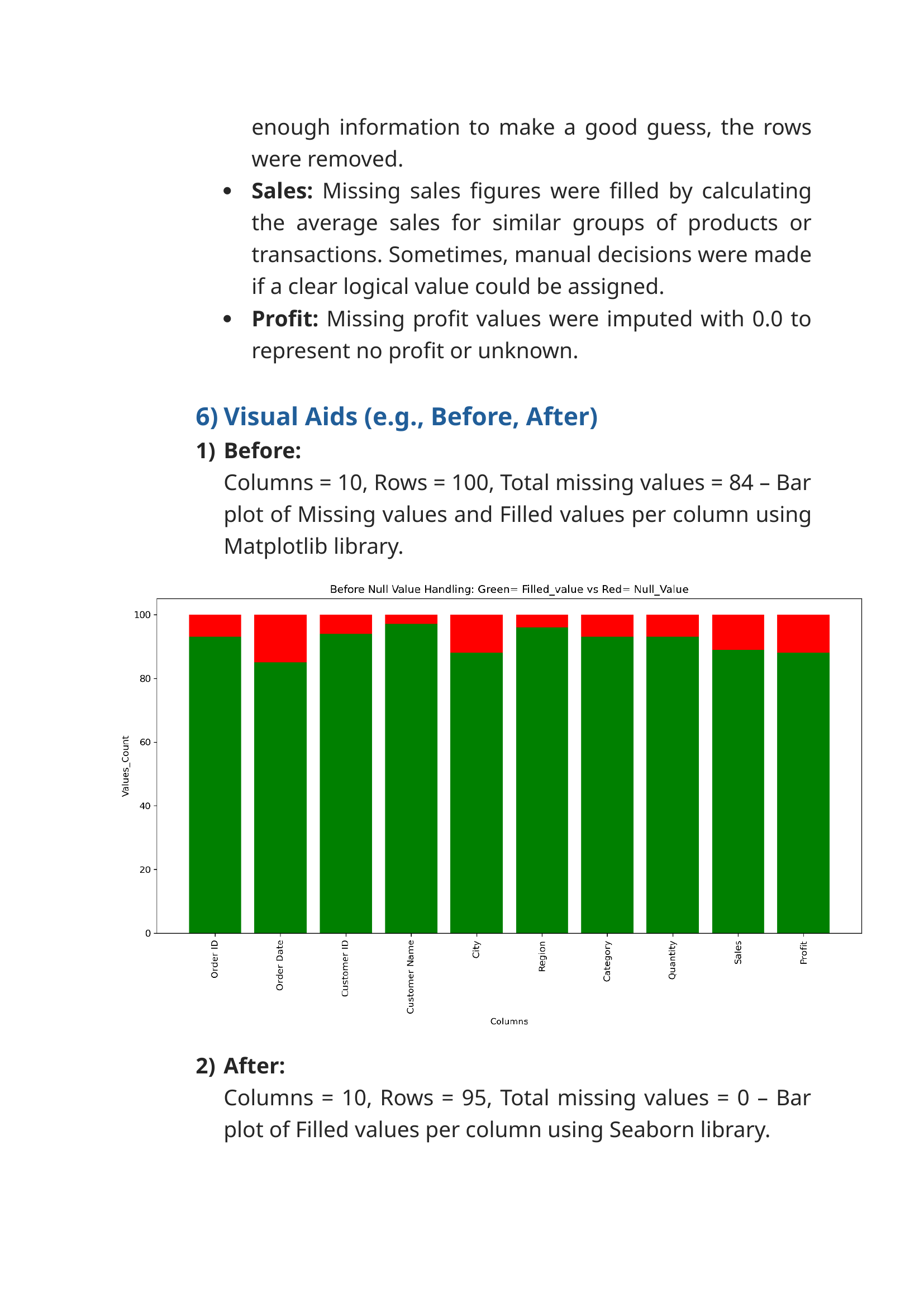
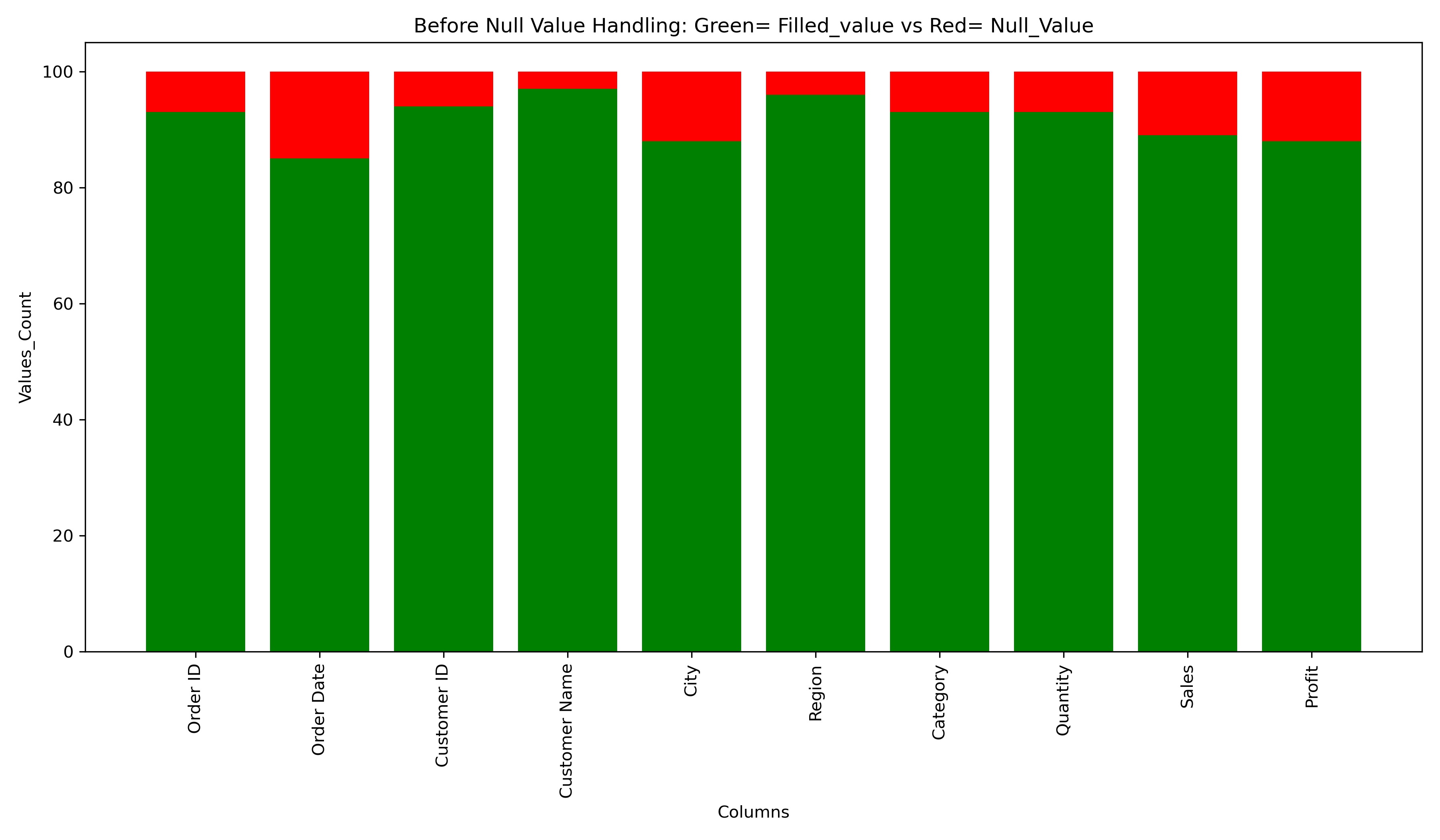
Before Handling null values
After Handling null values

Final Summary: Column wise Null value Handling Conclusion :

Before Handling null values

df_column = df.columns
df_column

cou = df.count()
df_count = cou.values
df_count

isnull = df.isnull().sum()
isnull_count = isnull.values
isnull_count

fig, ax = plt.subplots(figsize= (12,7))
ax.bar(df_column, df_count, color= "green")
ax.bar(df_column, isnull_count, bottom= df_count, color= "red")
ax.set_xlabel("Columns")
ax.set_ylabel("Values_Count")
plt.title("Before Null Value Handling: Green= Filled_value vs Red= Null_Value")
plt.xticks(rotation= 90)
plt.tight_layout()
plt.show()

df.info()

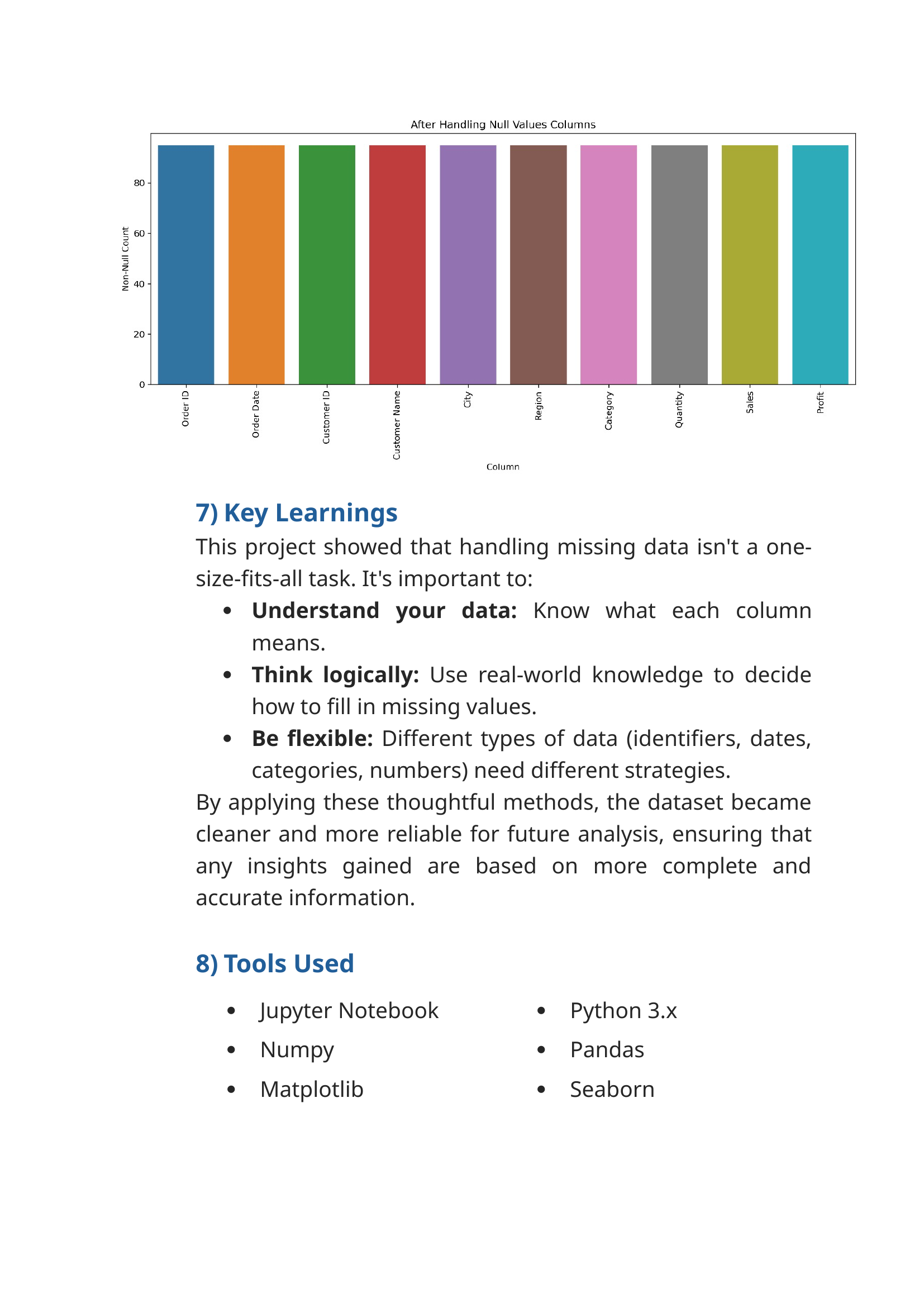
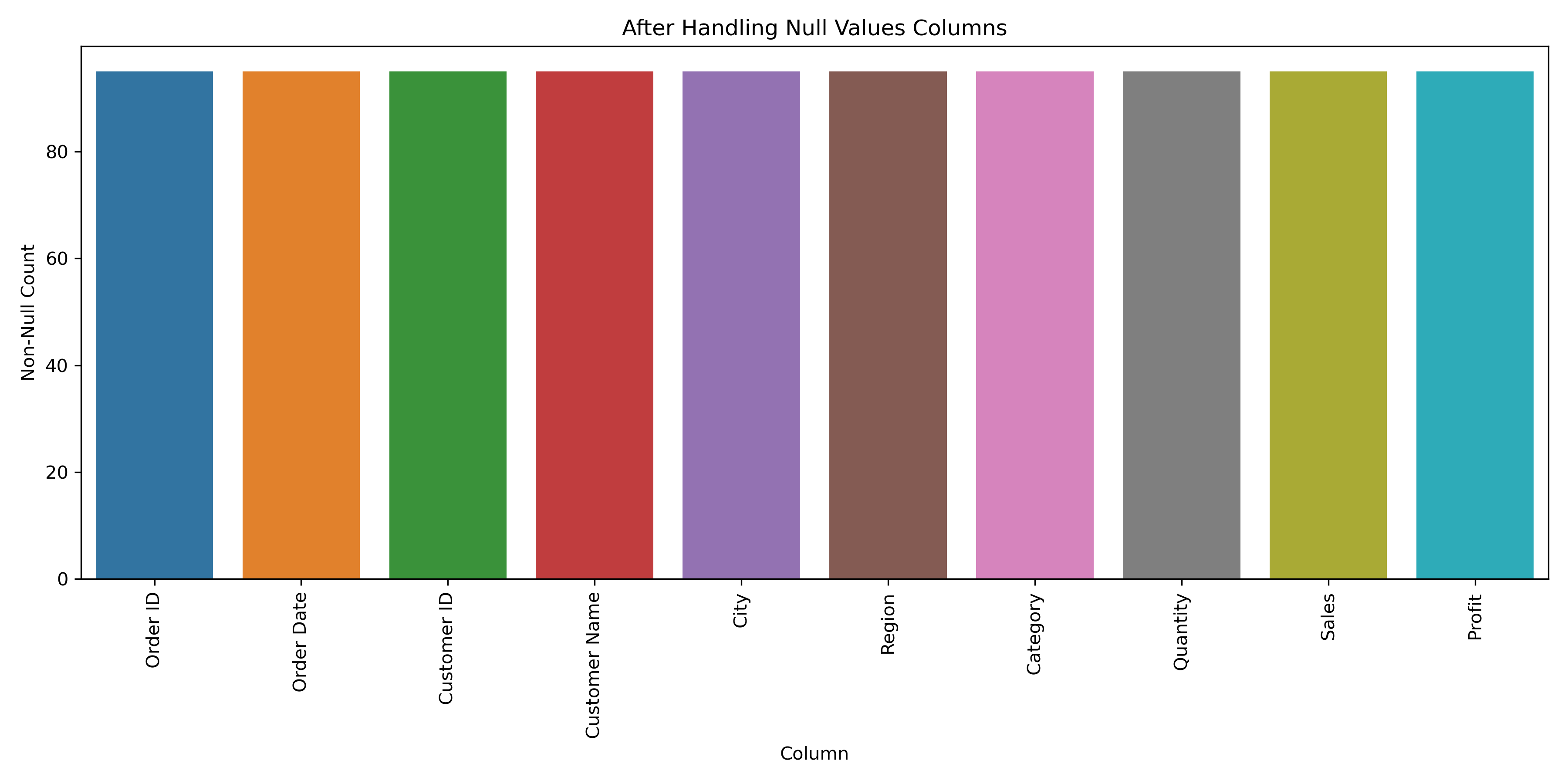
After Handling null values

df_handled_missing_values = pd.DataFrame(df_num)
df_handled_missing_values.head()

df_handled_missing_values.reset_index(drop= True, inplace= True)

non_null_counts = df_handled_missing_values.notnull().sum().reset_index()
non_null_counts.columns = ['Column', 'Non-Null Count']
plt.figure(figsize=(12, 6))
sns.barplot(data=non_null_counts, x='Column', y='Non-Null Count')
plt.title('After Handling Null Values Columns')
plt.xticks(rotation=90)
plt.tight_layout()
plt.show()

df_handled_missing_values.info()

Final Summary: Column wise Null value Handling Conclusion :

1) Order ID :

Filled with "Unknown" since all values are unique identifiers.

2) Customer ID :
Filled with "Unknown" due to uniqueness of values.

3) Customer Name :
Filled with "Unknown" since all names are unique and avoid misleading results.

4) Order Date :
Used category-region-date filtering, counting, and manual imputation based on realworld logic.

5) City :
Filled with "Unknown" — cities are all unique.

6) Region :
Filled based on city-to-region mapping; dropped one row.

7) Category :
Filled based on region-wise product frequency.

8) Quantity :
Used category-region-date filtering and manual imputation.

9) Sales :
Filled using group-based mean or manual logic. Some rows dropped.

10) Profit :
Nulls filled with 0.0 to avoid misleading results.

🛒 Walmart Null Value Handling Project Documentation

01_Walmart_Null_Values_Handling_Overall

🛒 Walmart Null Value Handling - Full Project Journal

Handling Null Values in Different Columns

Objective :

This is a realistic Walmart sales dataset. In this project, I aim to handle the missing (null) values using practical, real-world logic based on the type and context of each column.

Part 1:

Import the necessary libraries and dataset, then analyze the structure and quality of the data.

Part 2:

Apply appropriate real-world logic to impute.

Part 3:

Plot the chart before and after handling null values, Final summary.

PART - 1

Import the librarys and Dataset :

Dataset Analysis :

The dataset contains 10 columns and 100 rows. Based on the data types and usage, I’ve categorized the columns into 4 types:

Identifiers columns :

Order ID - 93 filled values & 7 null values,

Customer ID - 94 filled values & 6 null values,

Customer Name - 97 filled values & 3 null values.

Dates columns :

Order Date - 85 filled values & 15 null values.

Categorical columns :

City - 88 filled values & 12 null values,

Region - 96 filled values & 4 null values,

Categor - 93 filled values & 7 null values.

Numerical columns :

Quantity - 93 filled values & 7 null values,

Sales - 89 filled values & 11 null values,

Profit - 88 filled values & 12 null values.

PART - 2

1 - Handling the Identifiers columns :

1 - Handling the Order ID column :

Type: Object

Fill_values: 93

Null_values: 7

Order ID column Analysis :

Step - 1 :

I am looking for any same order id is there in the column. All 93 order are having a unique id.

Step - 2 :

Placing every order create unique Order ID. So, there is no possible to relate with any columns to fill the relative data for the missing value.

Conclusion :

Since the Order IDs are unique and there’s no meaningful logic to derive the missing values from other columns, I have filled the null values with the placeholder "Unknown" to retain row integrity without creating misleading data.

2 - Handling the Customer ID column :

Type: Object

Fill_values: 94

Null_values: 6

Customer ID column Analysis :

Step - 1 :

Checked for duplicate or repeated customer IDs to see if any customers placed multiple orders.

Result: All 94 customer IDs are unique.

Conclusion :

Since each customer is unique, there is no way to infer the missing values from other rows or columns. Therefore, I filled the null values with the placeholder "Unknown" to retain row integrity without creating misleading assumptions.

3 - Handling the Customer Name column :

Type: Object

Fill_values: 97

Null_values: 3

Customer Name column Analysis :

Step - 1 :

Checked for duplicate or repeated customer names to see if any customers placed multiple orders.

Result: All 97 customer names are unique.

Step - 2 :

Tried to relate Customer Name with Customer ID, but since all Customer IDs are also unique (except 6 missing), no reliable grouping or mapping is possible.

Conclusion :

As all customer names are unique and cannot be related to other identifiers, I filled the null values with the placeholder “Unknown” to preserve data consistency.

Why i did not use Forward Fill :

While forward fill is a valid approach, it can cause misleading data in this case.

2 - Handling the Dates columns :

1 - Handling the Order Date column :

Type: Object

Fill_values: 85

Null_values: 15

Order Date column Analysis :

Step - 1 :

Converted "Order Date" from object to datetime64[ns] using:

df_date["Order Date"] = pd.to_datetime(df_date["Order Date"], dayfirst= True)

Step - 2 :

Extracted Year and Month to analyze time-based distribution:

df_date["Year"] = df_date["Order Date"].dt.year

df_date["Month"] = df_date["Order Date"].dt.month

Step - 3 :

Since the Order IDs are unique and there’s no meaningful logic to derive the missing values from other columns, I have filled the null values with the placeholder `"Unknown"` to retain row integrity without creating misleading data.

Since each customer is unique, there is no way to infer the missing values from other rows or columns. Therefore, I filled the null values with the placeholder `"Unknown"` to retain row integrity without creating misleading assumptions.

Converted `"Order Date"` from object to datetime64[ns] using:

`df_date["Order Date"] = pd.to_datetime(df_date["Order Date"], dayfirst= True)`

Extracted `Year` and `Month` to analyze time-based distribution:

`df_date["Year"] = df_date["Order Date"].dt.year`

`df_date["Month"] = df_date["Order Date"].dt.month`

`df_date[(df_date["Year"] == 2025) & (df_date["Month"] == 1)].count()`

`df_date[(df_date["Year"] == 2025) & (df_date["Month"] == 1)].count()`

`df_date.groupby("Year").agg({"Month" : "count"})/df_date["Year"].count()*100`

`df_date.at[99, "Order Date"] = "2025-01-23"`

Checked Upon reviewing the `City` column, I found that all 88 filled values are unique — no city names are repeated across the dataset. Due to this uniqueness, there is no meaningful way to relate or group missing values with other categorical columns such as Region or Categorie.

In this scenario, using `'Unknown'` to fill the 12 missing city values is the most appropriate and logical choice.

Using `'Unknown'` ensures data integrity without distorting analytical results.